
This post is part of a series of articles written by 2018 Summer of Maps Fellows. Azavea’s Summer of Maps Fellowship Program is run by the Data Analytics team and provides impactful Geospatial Data Analysis Services Grants for nonprofits and mentoring expertise to fellows. To see more blog posts about Summer of Maps, click here.
Have you ever spent too much time tracing outlines of images in ArcMap? And the quality of the traced data is not even as good as it could be? Do you wish there were tools to automate that process? I totally understand. I have been there.
Manually digitizing maps can be tedious and inaccurate, knowing how to automate the process using ArcMap and R saves a lot of time and can increase the accuracy. This blog provides an approach that uses image processing and remote sensing techniques in R and ArcGIS to digitize image maps – the kind often found in a PDF that provides no way to get at the underlying data. The final output will be georeferenced raster or vector spatial datasets.
Project background
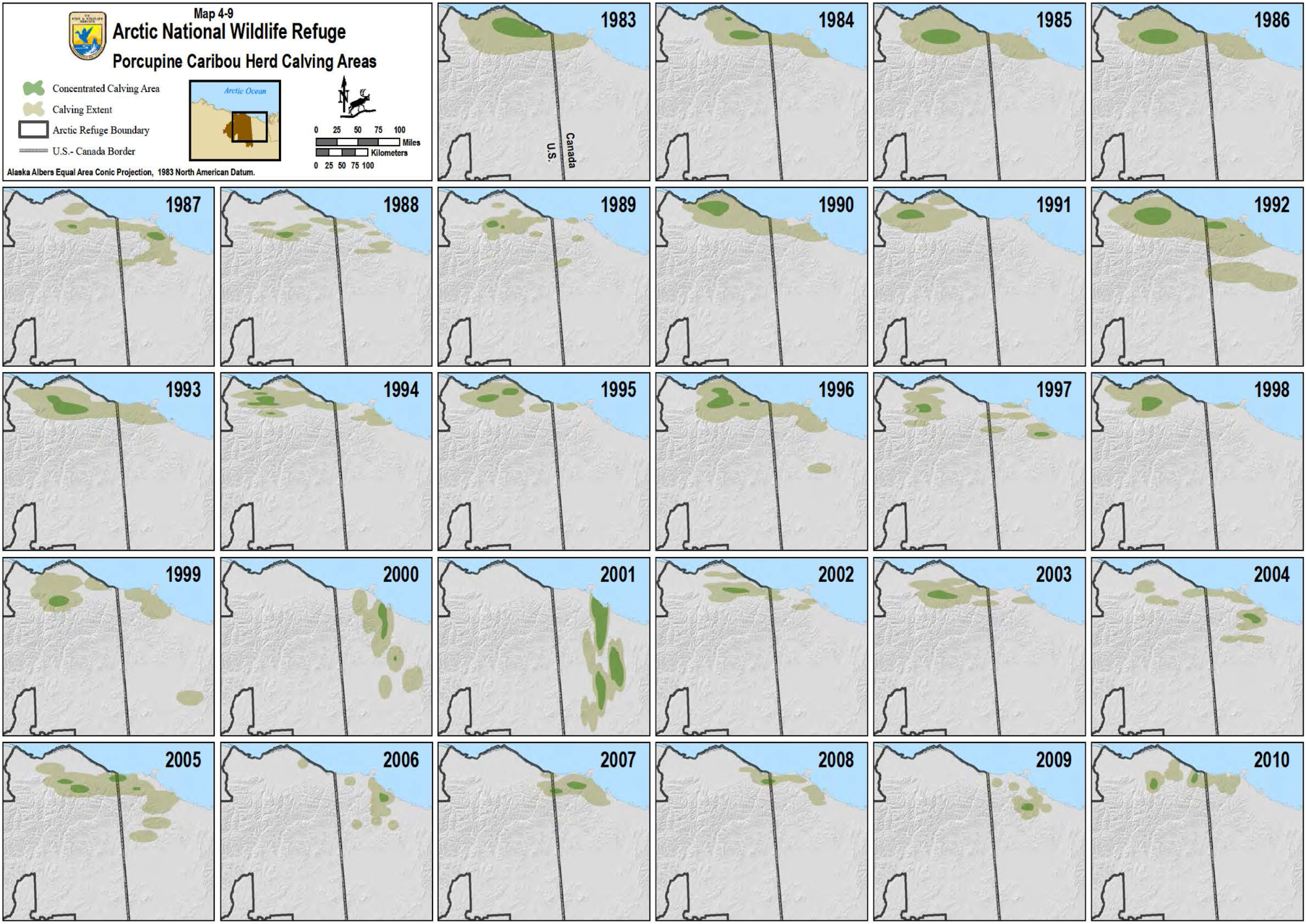
This summer I worked with Audubon Alaska to complete an ecological analysis of the Arctic National Wildlife Refuge. In this blog, I’ll walk through the process I used to extract data from a historic map of porcupine caribou herd calving areas.
Caribous are migratory animals that return to specific locations (calving areas) every spring where pregnant females give birth. Although the highest density calving areas may vary from year to year, caribou return to the same general broader areas, making it important to keep track of both annual variation and inter-annual patterns.
General Process
The general process of digitizing one map includes five steps: crop the image, georeference, image classification, extract the shapes, and smooth the polygons.
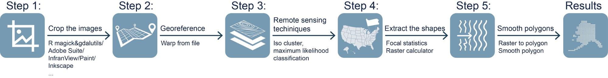
I included both R and ArcPy code in the descriptions below. Note that you can automate the entire process using batch processing and ModelBuilder in ArcMap.
Step 1: Crop the image
If you only have one historic map and it is in the correct extent you hope to digitize, you are welcome to skip to Step 2. Otherwise, there is a little preparation work to make sure you are only digitizing your map in your area of interests which will also save you a lot of time. There are a lot of graphic design software tools for editing images, for example, Adobe Creative Cloud, IrfanView, Paint, Inkscape, etc. I use the open source tools available in R.You can adjust contrast, lightness, and saturation first using an R package, magick, then crop your image, split images into separate files, and export them into different formats using another package gdalUtils.
library(magick)
# Read the image, change brightness, saturation and hue
caribou <- image_read('D:/AA/forblog/caribou.png', density = NULL, depth = NULL, strip = FALSE)
caribou1 <- image_modulate(caribou, brightness = 120, saturation = 100, hue = 200)
# Export the image in any format
image_write(caribou1, path = "caribou.png", format = "png")
# Try to split the image automatically
library(gdalUtils)
# Get the dimensions of the jpg
dims <- as.numeric( strsplit(gsub('Size is|\\s+', '', grep('Size is', gdalinfo('caribou.png'), value=TRUE)),  ',')[[1]])
# Set the separate image size, width and height
incrx <- 750
incry <- 637
# Create a data.frame for cutting the image and the corresponding output filenames.
xy <- setNames(expand.grid(seq(0, dims[1]-incrx, incrx), seq(dims[2], incry, -incry)),
              c('llx', 'lly'))
xy$nm <- paste0(c(seq(2005, 2010, 1),seq(1999, 2004, 1),seq(1993, 1998, 1),seq(1987, 1992, 1),seq(1981, 1986, 1)), '.png')
name <- c(seq(2005, 2010, 1),seq(1999, 2004, 1),seq(1993, 1998, 1),seq(1987, 1992, 1),seq(1981, 1986, 1))
# Create a function to split the raster using gdalUtils::gdal_translate
split_rast <- function(infile, outfile, llx, lly, win_width, win_height) {
 library(gdalUtils)
 gdal_translate(infile, outfile,
                srcwin=c(llx, lly - win_height, win_width, win_height))}
mapply(split_rast, 'caribou.png', xy$nm, xy$llx, xy$lly, 750, 637)
Step 2: Georeference the images

Scanned maps and PDFs of historical data usually do not contain spatial reference information. Hence you will need to georeference your map before digitizing it. In this step, I will use the georeference toolbar in ArcMap. You can add a base map layer or some other dataset with coordinates to get the context when you assign the coordinate system to the map frame.
If you have a series of maps of the same location, saving the links to a text file will be very helpful. You can then use the .txt file in the warp from file tool for batch processing, and then write ArcPy code or ModelBuilder model to automate the process. Here is the example of using ArcPy, you can replace the names of the files and run it in the Python Window in ArcCatalog:
import arcpy, os
arcpy.env.workspace = r"D:\blog\forblog\infolder"
OutF = r"D:\blog\forblog\outfolder"
Ext = ".jpg"
LinkFile = r"D:\blog\forblog\reference.txt"
ListRas = arcpy.ListRasters()
for ras in ListRas:
    basename = arcpy.Describe(ras).baseName
    outpath = os.path.join(OutF, basename + Ext)
    arcpy.WarpFromFile_management(ras, outpath, LinkFile, transformation_type="POLYORDER1", resampling_type="NEAREST")
    print "Georeferenced {} successfully".format(basename)
Step 3: Iso cluster and maximum likelihood classification
Iso cluster performs clustering of the multivariate data in the list of input raster. The specified number of classes value is the maximum number of the clusters that can result from the clustering process. The optimal number of classes should be greater than two but is usually found after testing some numbers, analyzing the resulting clusters and retrying the function. Maximum likelihood classification tool will then use the signature file produced from Iso Cluster to produce the optimal number of classes in an output raster.
If you have a series of maps using the same color theme, the shape you hope to extract from the maps will have the same value in each final output raster. Here is the code in ArcPy:
import arcpy, os

arcpy.env.workspace = r"D:\blog\forblog\outfolder"

OutF = r"D:\blog\forblog\isocluster"

arcpy.gp.IsoCluster_sa("2010.jpg", "D:\blog\forblog\signature.GSG", "10", "20", "20", "10")

print "Iso cluster {} successfully".format(basename)

ListRas = arcpy.ListRasters()

for ras in ListRas:

     basename = arcpy.Describe(ras).baseName

     outpath = os.path.join(OutF, basename)

     arcpy.gp.MLClassify_sa(ras, "D:\blog\forblog\signature.GSG", outpath, "0.0", "EQUAL", "", "")

     print "Iso clustered {} successfully".format(basename)
Step 4: Extract the shapes
You now have the output raster from ArcMap, the next step is to extract the shapes. I recommend you use focal statistics tools before you use raster calculator to extract them into a new raster file because they usually have rough edges. For example, you can use focal statistics majority and circle neighborhood to smooth the shapes. Depending on the data you have, you can try with a smaller radius but do it multiple times until you get a satisfying result. After this, you can use raster calculator to extract the shapes you want into a new raster.
import arcpy, os, numpy

arcpy.env.workspace = r"D:\blog\forblog\isocluster"

focalstatsF = r"D:\blog\forblog\focalstats"

generalF = r"D:\blog\forblog\gen"

concentF = r"D:\blog\forblog\conc"

ListRas = arcpy.ListRasters()

for ras in ListRas:

    basename = arcpy.Describe(ras).baseName

    focaloutpath = os.path.join(focalstatsF, basename)

    generaloutpath = os.path.join(generalF, basename)

    concentoutpath = os.path.join(concentF, basename)

    arcpy.gp.FocalStatistics_sa(ras, focaloutpath, "Circle 12 CELL", "MAJORITY", "DATA")

    newGrid = arcpy.sa.Reclassify(focaloutpath, "VALUE", "1 NODATA;2 NODATA;3 NODATA;4 1;5 NODATA;6 1;7 NODATA;8 NODATA", "DATA")

    newGrid.save(generaloutpath)

    newGrid = arcpy.sa.Reclassify(focaloutpath, "VALUE", "1 NODATA;2 NODATA;3 NODATA;4 2;5 NODATA;6 NODATA;7 NODATA;8 NODATA", "DATA")

    newGrid.save(concentoutpath)

    print "General and concentrated area raster {} successfully".format(basename)
Step 5: Export and Smooth polygon
If you want the final result to be shapefiles, here is one more step after you get the raster files in using raster to polygon tool. You can then play with the smooth polygon tool to smooth the boundary.
import arcpy, os

   arcpy.env.workspace = r"D:\blog\forblog\gen"

   PolyF = r"D:\blog\forblog\genpoly"

   ListRas = arcpy.ListRasters()

   for ras in ListRas:

        basename = arcpy.Describe(ras).baseName

        Polyoutpath = os.path.join(PolyF, basename)

        arcpy.RasterToPolygon_conversion(ras, Polyoutpath, simplify="SIMPLIFY", raster_field="VALUE")

import arcpy, os

   arcpy.env.workspace = r"D:\blog\forblog\genpoly"

   smooF = r"D:\blog\forblog\smopoly"

   files = arcpy.ListFeatureClasses()

   for shp in files:

        basename = arcpy.Describe(shp).baseName

        smoooutpath = os.path.join(smooF, basename)

        arcpy.SmoothPolygon_cartography(shp , smoooutpath, algorithm="PAEK", tolerance="20000 Unknown", endpoint_option="FIXED_ENDPOINT", error_option="NO_CHECK")

/ for concentrated area

import arcpy, os

    arcpy.env.workspace = r"D:\blog\forblog\conc"

    PolyF = r"D:\blog\forblog\conpoly"


     ListRas = arcpy.ListRasters()

     for ras in ListRas:

         basename = arcpy.Describe(ras).baseName

         Polyoutpath = os.path.join(PolyF, basename)

         arcpy.RasterToPolygon_conversion(ras, Polyoutpath, simplify="SIMPLIFY", raster_field="VALUE")
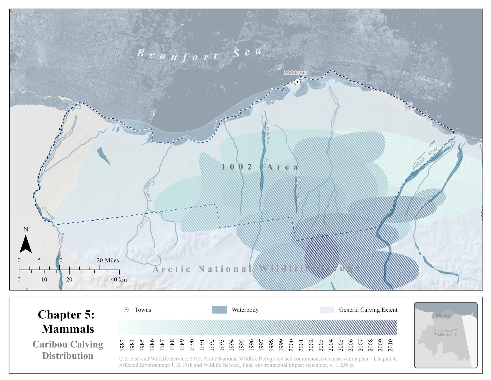
Here are the smoothed polygons of caribou calving extent (Image 2):
If you finished all the steps, congratulations, you have successfully digitized your maps! Here is a map showing the historical distribution of caribou in one map.
Other options
This blog is only an exploratory approach to demonstrate how to digitize non-georeferenced maps into geospatial datasets. I choose to georeference first and then do classification in ArcMap. There are still a lot of other ways, for example, you can extract shapes into vectors using Image Trace tool in Adobe Illustrator and then georeference the vector data in ArcMap. That will make the editing process easier but might be harder to automate if you have a series of maps.
Have you completed a similar workflow to digitize data from images or PDFs? Reach out to us on Twitter and let us know how you did it!
If you’re interested in applying for a 2019 Summer of Maps fellowship position, sign up to receive notifications about future opportunities.