Preparing Data for MaxEnt Species Distribution Modeling Using R

This post is part of a series of articles written by 2018 Summer of Maps Fellows. Azavea’s Summer of Maps Fellowship Program is run by the Data Analytics team and provides impactful Geospatial Data Analysis Services Grants for nonprofits and mentoring expertise to fellows. To see more blog posts about Summer of Maps, click here.

Species distribution modeling requires two sets of data inputs: presence points and environmental data related to the species of interest. This blog post describes how to use R to turn disparate environmental data into clean, usable raster data that can be fed into a MaxEnt species distribution model.

What is species distribution modeling?

Before we dive into the data-cleaning code, we need to understand why properly-formatted data is essential for modeling.

Species distribution modeling is a type of spatial analysis used to find likely locations of any given species. Say that you want to understand where in a jungle a rare monkey species lives; a species distribution model would take the information you have, and turn it into a single map that shows the likely range of where the monkeys live.

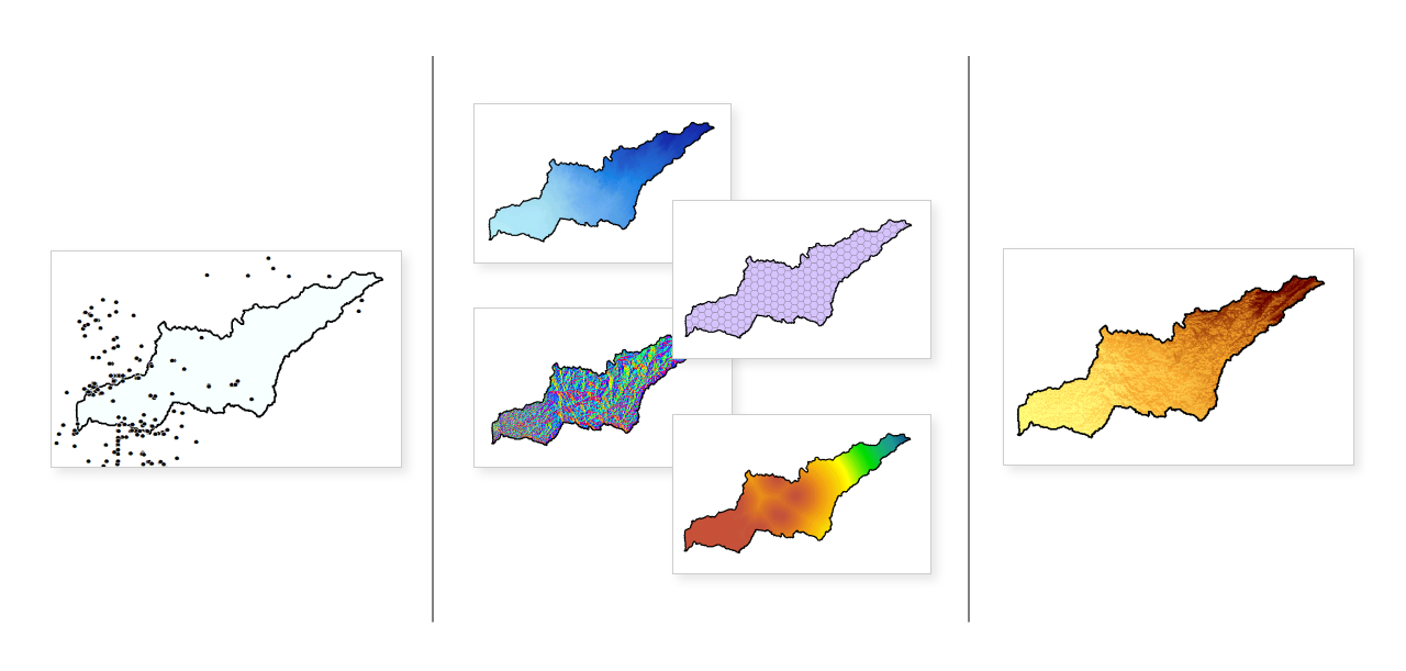
There are two types of data necessary to build a species distribution model (SDM). First, you need presence points, also called observation points or occurrence points. These are exactly what they sound like – points where the species is known to have been seen or live. The more you have, the better, but many species distribution models can work successfully with as few as 10-15 presence points.

Secondly, an SDM requires you to have environmental data for the area you’re studying. This could include things like elevation, precipitation, land cover, forest type, and so forth. Again, the more data, the better, but SDMs can run well with only 2 or 3 environmental variables.

Environmental data often requires significant cleaning before it can be used in an SDM because it comes in many different formats and from many different sources. There are several types of SDMs – the strategy for data-cleaning depends on the model. In this case, we’ll work through data preparation for a MaxEnt SDM.

Using the MaxEnt GUI and finding data

MaxEnt stands for Maximum Entropy distribution modeling. For this demonstration, I used the MaxEnt Graphical User Interface, a Javascript application that can be downloaded here.

The MaxEnt software comes with a useful PDF manual that describes how to use the software itself, so that information will not be repeated in this post. Instead, it will cover what the MaxEnt manual does not – how to prepare your data for use in MaxEnt.

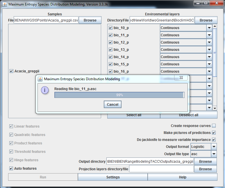
MaxEnt requires that environmental variables meet the following criteria:

A .asc or .ascii format
All environmental variables are identical in resolution, extent, and projection

The quickest way to make your data meet those two criteria is to use an R script that can take a variety of environmental data inputs and create data which will work for MaxEnt.

An R Script for Preparing Data for MaxEnt

There are five steps required in the script to prepare your data for use in MaxEnt.

Set up your R packages and libraries
Set up some parameters you’ll use to make your data uniform
Read your data into R
Resample and extend your data using the parameters from step 2
Write your data out into a .asc format

Let’s go through these steps one by one.

The first step is required to give us the tools we need to manipulate, read, and write spatial data in R. The packages we need are raster, rgdal, sf, tidyverse, and fasterize. The code below shows how to get them set up at the start of the script:

# install necessary packages and libraries
install.packages("raster")

install.packages("rgdal")

install.packages("sf")

install.packages("tidyverse")

install.packages("fasterize")

library(sf)

library(raster)

library(rgdal)

library(tidyverse)

library(rgeos)

library(scales)

library(fasterize)

Once the necessary packages are set up, it’s time to create a parameter that we’ll use throughout the rest of the script. We’ll need a projection that all of our data can be set to – the easiest one to use for MaxEnt is a simple lat/long projection using WGS 1984. (In fact, lat/long isn’t really a projection, but rather an unprojected way of displaying data, but that’s not really worth getting into). The code needed to do this looks like this:

# set up projection parameter for use throughout script

projection <- "+proj=longlat +ellps=WGS84 +datum=WGS84 +no_defs"

The second parameter needed is an extent parameter. Unlike for projection, I can’t recommend a certain extent. The extent is simply a set of numbers that define the rectangular area your data will cover. What those numbers are depends where in the world your data is located. To create an extent object parameter, use code like this:

#set up extent parameter for use throughout script

ext <- extent(-180, 180, -90, 90)

That code will result in an extent that covers the whole world, from 180 degrees West to 180 degrees East and 90 degrees North and South. Choose an extent that covers your whole study area and is slightly more extensive than your most extensive dataset. Although extents don’t always have to be in degrees of latitude and longitude, for this example, they should be, because this example uses a lat/long projection parameter.

Now, we’re going to walk through the next two steps – first, for your raster datasets, and second, for any vector environmental datasets you may have. Raster and vector data has to be treated differently in R and most other geospatial work. Therefore, the script needed to read in and manipulate a raster dataset will be different from that used for a vector dataset.

Let’s start with a raster dataset, taking, say, elevation as an example. Elevation is a commonly used environmental variable in species distribution models. Before you try to read in any data, make sure your R working folder is set to the location you keep your data. R can read in many types of raster data, but generally, a TIFF is easiest to work with. Let’s take a look at the full code for reading in and manipulating the elevation data, and then break it down.

#process for Environmental Variable 1 - Elevation

# read in raster data

assign(paste0("elev_", "raw"), raster(“elevation.tif”))

# reproject to our shared parameter

assign(paste0("elev_", "projected"),

projectRaster(elev_raw, crs=projection))

# create variable equal to final raster

assign(paste0("elev_final"), elev_projected)

# extend elev_final to the desired extent with NA values

elev_extended <- extend(elev_final_x, ext, value=NA)

The first part of this script takes data from your computer and reads it into R. The name of the data to be read in is given by “elevation.tif” – be sure to use the full filenames for your data, enclosed in quotes, as seen here. I use that data to create an R raster object called elev_raw.

The second section of code reprojects elev_raw using the parameter we created and makes that into a new raster object, elev_projected. Then we rename elev_projected to elev_final, and extend elev_final to our extent parameter and call that elev_extended. The “gaps” between our elevation dataset’s original extent and our chosen “ext” extent are filled in by NA values so that they do not distort the data.

Now let’s take a look at the code necessary to read in and manipulate data that is in vector format:

# process for Environmental Variable 2 - Vegetation Community

#read in spatial data

assign(paste0(“vegcommunity, "_raw"),

sf::st_read(dsn="FOLDER NAME", layer=”vegcommunity”))

# convert new spatial vector data to raster

require(raster)

hold.raster <- raster()

extent(hold.raster) <- extent(vegcommunity_raw)

res(hold.raster) <- 20

assign(paste0("veg", "_rasterized"),

fasterize(vegcommunity_raw, hold.raster, ‘ATTRIBUTE’))

# reproject to our shared parameter

assign(paste0("veg_", "projected"),

projectRaster(veg_rasterized,crs=projection))

# create variable equal to final raster

assign(paste0("vegcommunity_final"), veg_projected)

Before using this script, place your vector data in a separate folder within your working folder. In this case, I called it “FOLDER NAME”. This is to simplify the reading-in process in the first section of the code. The layer=”vegcommunity” line does not include the files .shp or other extension intentionally – this will cause an error in the script for vector data.

The second section of this code is the rasterizing process. Before the actual rasterization, you have to set up a raster dataset to fill in with the data you’re about to rasterize, which is what the first 4 lines do. Then the old object vegcommunity_raw is rasterized into veg_rasterized. The ATTRIBUTE section of the code tells the rasterization function on which attribute to rasterize. Vector layers can have many different attributes – pick the one that’s relevant to you and type the name of the attribute table column in place of ATTRIBUTE.

In the third section, veg_rasterized is re-projected, and in the final section, renamed to vegcommunity_final.

Although the processes for raster and vector data are different, each of these sections of code can be copied and repeated for each of your variables as long as you change the object names each time.

After you have finished reading in, manipulating, rasterizing, and renaming all of your variables, it is time to resample and re-extend them. Let’s say that in addition to elevation and vegetation community, you also have variables for landcover, precipitation, and slope.

Therefore, you currently have 5 raster objects – elev_final, vegcommunity_final, landcover_final, precip_final, and slope_final. However, they may all have different spatial resolutions, even though they all share the same projection.

Pick one of your variables to use as a basis for resampling. This means that the others will all be forced to share its resolution. If you aren’t worried about processing time and don’t mind larger file sizes, pick the variable with the smallest pixels (highest resolution). If you want quick processing and small files, pick the variable with the largest pixels. In this case, I’ll choose elev_final as my basis for resampling.

landcover_final_re <- resample(landcover_final, elev_final)

precip_final_re <- resample(precip_final, elev_final)

slope_final_re <- resample(slope_final, elev_final)

vegcommunity_final_re <- resample(vegcommunity_final, elev_final)

elev_final_re <- resample(elev_final, elev_final)

(It’s not strictly necessary to resample elev_final to itself, but it’s good practice to treat all your variables equally, even when one of them is being used as a basis for the others.) Next, we have to re-extend the datasets to make sure that their shared extent was not influenced by the resampling.

landcover_tend <- extend(landcover_final_re, ext, value=NA)

precip_tend <- extend(precip_final_re, ext, value=NA)

slope_tend <- extend(slope_final_re, ext, value=NA)

veg_tend <- extend(vegcommunity_final_re, ext, value=NA)

elev_tend <- extend(elev_final_re, ext, value=NA)

Now we have five datasets that are identical in extent, resolution, and many other properties. Our final step is to write out these environmental datasets into the .asc format that the MaxEnt GUI uses.

writeRaster(landcover_tend, filename=”landcover_output.asc”, format=’ascii’, overwrite=TRUE)

writeRaster(precip_tend, filename=”precip_output.asc”, format=’ascii’, overwrite=TRUE)

writeRaster(slope_tend, filename=”slope_output.asc”, format=’ascii’, overwrite=TRUE)

writeRaster(veg_tend, filename=”veg_output.asc”, format=’ascii’, overwrite=TRUE)

writeRaster(elev_tend, filename=”elev_output.asc”, format=’ascii’, overwrite=TRUE)

Congrats! Your environmental datasets should now be sitting in your working folder, ready for use in the MaxEnt GUI.

Species distribution modeling in the Bear River Watershed

I used this process, and the MaxEnt GUI, in my work this summer in Azavea’s Summer of Maps program. Summer of Maps pairs geospatial students like myself with nonprofits like the Sierra Streams Institute (SSI). The Sierra Streams Institute is a habitat conservation and restoration organization that works in the Bear River Watershed of California, northeast of Sacramento.

Sierra Streams prioritized 10 different species for species distribution modeling, including plants, birds, reptiles, and one mammal species, the Sierra Nevada Mountain beaver. By using R to prepare the data, MaxEnt to analyze it, and ArcGIS to create attractive visualizations of it, I was able to help SSI understand their 10 top priority species.

Useful links for getting answers about species distribution modeling, MaxEnt, and R scripting

Although the MaxEnt GUI enables creation of a SDM , the learning curve associated with using the program can be steep. I hope you’ll be able to save valuable time on data preparation by using this blog as a guide.

There are also many other helpful resources on the web regarding species distribution modeling in general, the MaxEnt algorithm specifically, and how to write and use R scripts: