Evaluating Machine Learning Models in R: Predicting Marine Debris

This post is part of a series of articles written by 2018 Summer of Maps Fellows. Azavea’s Summer of Maps Fellowship Program is run by the Data Analytics team and provides impactful Geospatial Data Analysis Services Grants for nonprofits and mentoring expertise to fellows. To see more blog posts about Summer of Maps, click here.

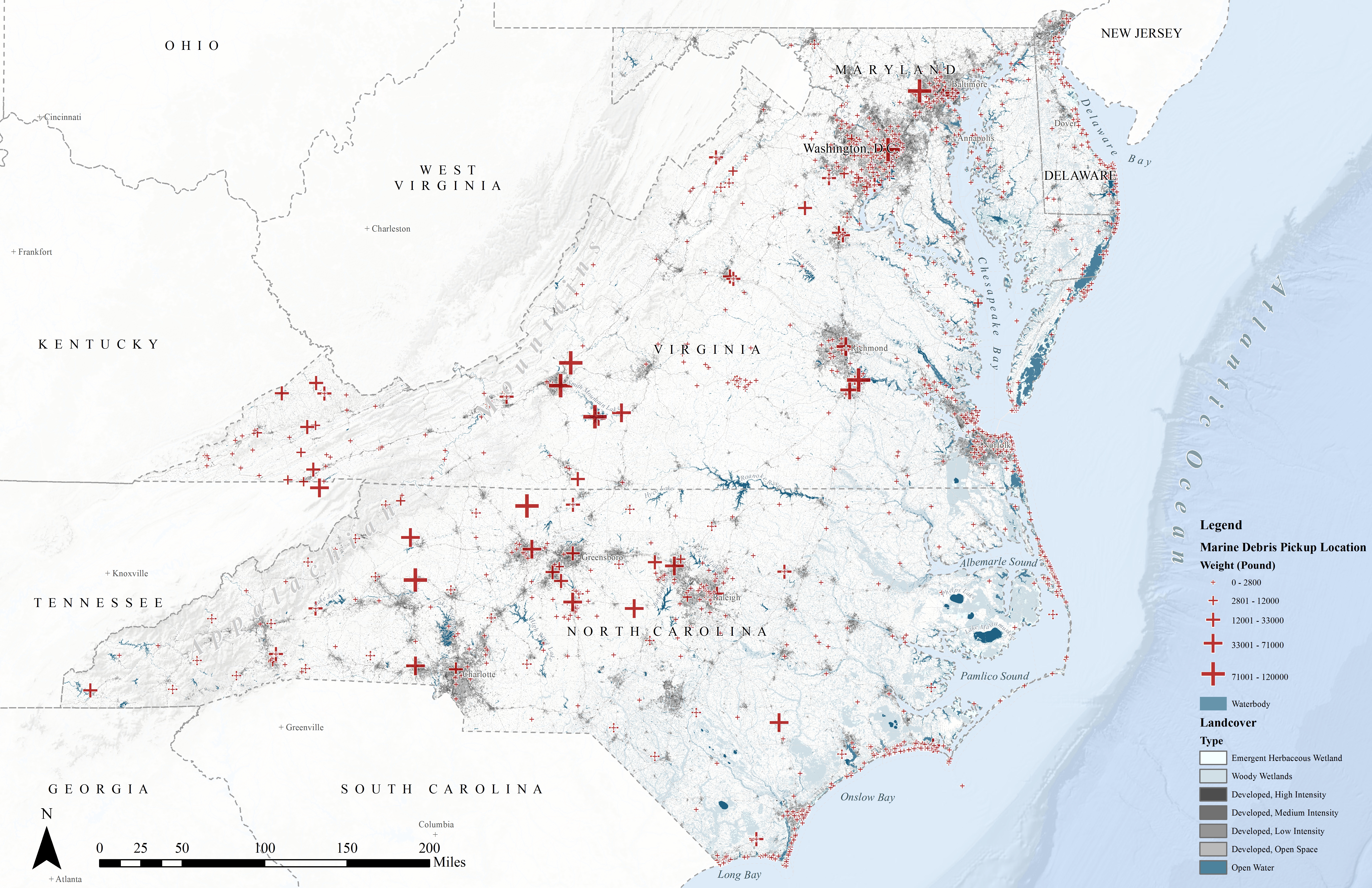
This blog post is based on the project I worked with National Aquarium, Identifying Patterns in Mid-Atlantic Marine Debris. The main dataset of this project came from the International Coastal Cleanup (ICC) events. The dataset has 2840 records from 2008 to 2015 after data cleaning. Below is a map displaying all the cleanup records onto one map. Each cross represents one clean up event. It is obvious that the cleanup events cluster at the urban area. That is to say, the dataset bias towards urban development. Although there are no crosses at some locations, that does not mean there are no marine debris. It might just because there were no people examining the area.

Weight of collected marine debris, by location of clean-up

Many geospatial analysis models, for example, generalized linear model and geostatistical regression, assume all variables are normally distributed. However, the dependent variable, the weight of marine debris in this dataset, has to be log transformed to fit this assumption. In this case, Machine learning models might be better options to deal with this dataset because they usually do not require sampling techniques or normalizing.

Exploratory Data Analysis – Marine Debris and Independent Variables

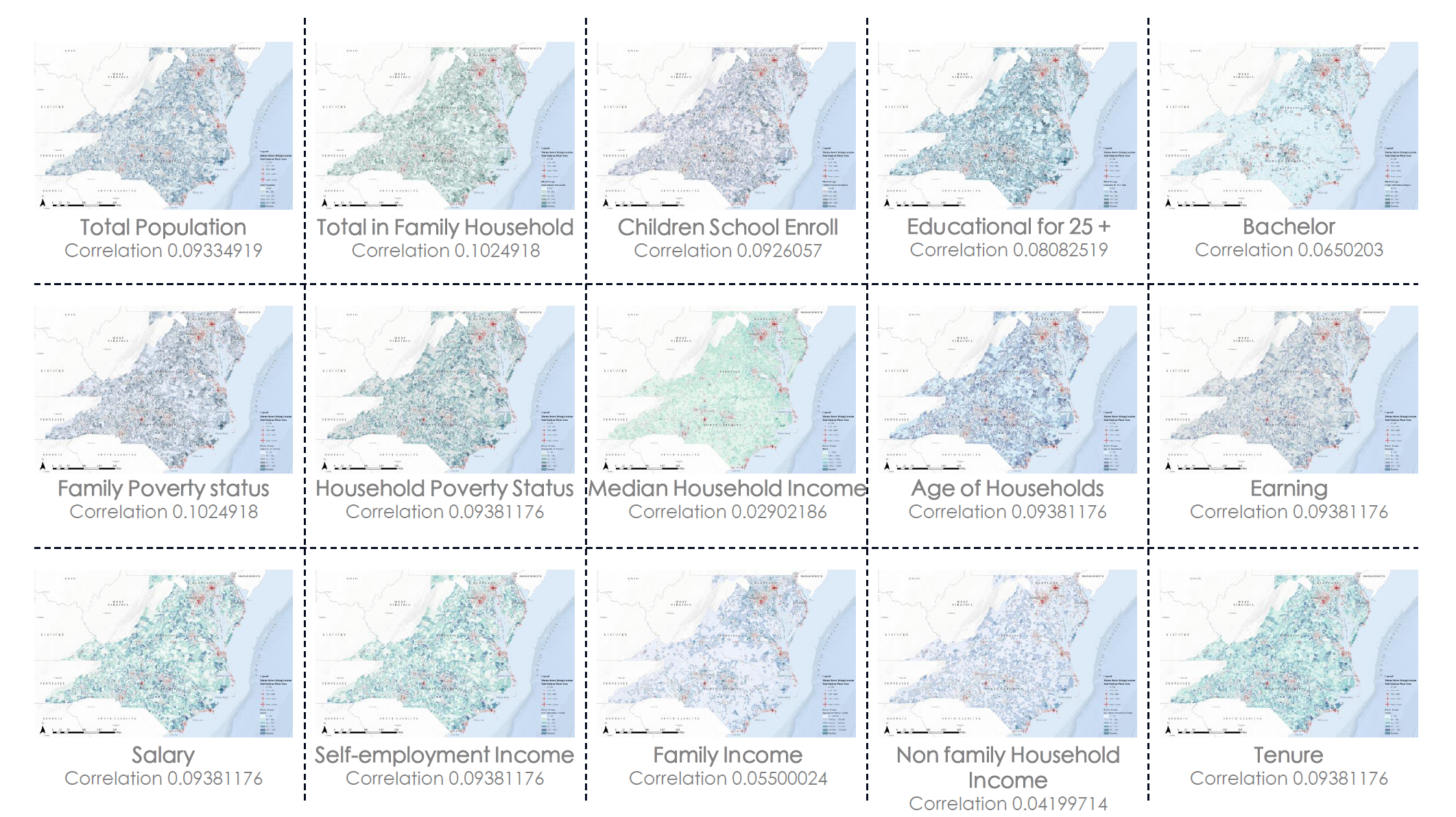
Here is a matrix showing all the Pearson correlation coefficients between the dependent variable, Pounds of Marine Debris (Pounds), and all the social-economic independent variables. The Pearson correlation value is only an indicator of the linear correlation between variables. As we can see in the image below, the correlation is not really strong, therefore, the generalized linear models might fail in describing the underlying spatial pattern of marine debris.

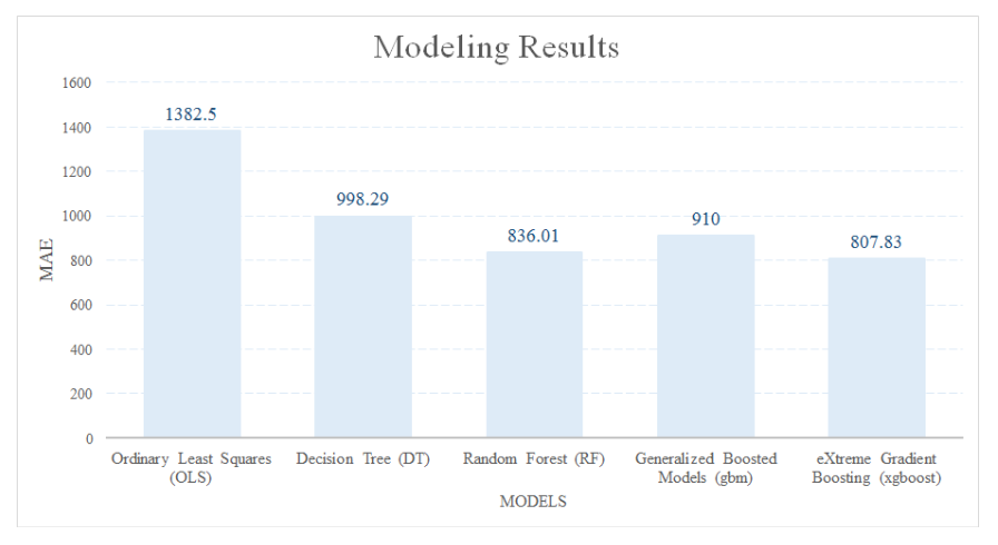
Mapping the independent census variables against marine debris data

Modeling

To compare with the linear regression models, for example, Ordinary Least Squares (OLS), I tried four other machine learning approaches, including Decision Tree (DT), Random Forest (RF), Gradient Boosting Models (gbm) and eXtreme Gradient Boosting (xgboost). The training dataset and the testing dataset is divided by 80：20. Since the dependent variable is continuous, I used mean absolute error (MAE) to evaluate and compare the models.

Here is the code in R of separating the training dataset and testing dataset. I used createDataPartition in caret. You can also use other packages like cvTools in R to split the training dataset and testing dataset.

library(dplyr)
library(tidyverse)
library(sf)
library(caret)

points <- st_read("C:/Users/dell/Box Sync/SOM/Aquarium/WP/points_extractvalue/points_extractvalue0818.shp") %>% 
  as.data.frame() %>% 
  dplyr::select(c(Pounds, TotalItems, TotalSinPl, itemspermi, singplaper, poundsperm, Forjoin,
                  TtlPp, TtlIn, SCHOO, EDUCA, BACHE, POVERTYSTA,
                  POVERTYS_1, MEDIA, AGEOF, EARNI, SALAR, SELFE, 
                  AGGRE, NONFA, TENUR, VACAN, MORTG, PopDen, dis2water, slope_re,
                  hillshade_, landcover, DEM)) %>% 
  mutate(landcover = as.factor(landcover))

x_train1 <- points[1:2840,]
x_train1 <- x_train1 %>% 
  dplyr::select(-c(Pounds,TotalItems,TotalSinPl,itemspermi,singplaper,poundsperm,Forjoin))
y_train1 <- points$Pounds 

## 80 / 20 split
set.seed(777)
partition1 <- createDataPartition(y_train1,p=.8,list=F)
training1 <- x_train1[partition1,]
testing1 <- x_train1[-partition1,]
y_test1 <- y_train1[-partition1]

1. Ordinary Least Squares (OLS)

OLS is one typical representative of the linear regressions. OLS generally fits a function with the data by minimizing the sum of squared errors. You can use the Metrics package in R. The OLS prediction result on the testing dataset has an MAE of 1382.50. I will use this number to compare across all the other models.

library(Metrics)
fit_ols <- lm(Pounds ~ ., data=cbind(training1,Pounds=y_train1[partition1]))
summary(fit_ols)
y_hat_ols <- predict(fit_ols,testing1)

print(paste("OLS", mae(y_test, y_hat_ols)))

2. Decision Tree (DT)

DT is a type of supervised learning algorithm that can be used in both regression and classification problems. It works for both categorical and continuous input and output variables. You can use the rpart package in R.

DT can be built and interpreted easily and it also performs well on discrete variables.

The disadvantage of DT is it tends to overfit training set. When the dataset has too many noises or is sampled in a wrong way, DT will learn “too much” from the dataset. To improve the single DT performance, pruning and limiting the tree’s height may be applied.

The decision tree prediction result on the testing dataset has an MAE of 998.29, which is a lot improved from the generalized linear regression.

library(rpart)
## Rpart is similar to 'tree' but much faster, as parts of its code is writen in C
## for classification, set method = "class"
fit_tree <- rpart(Pounds ~ .,
                  method="anova", data=cbind(training1,Pounds=y_train1[partition1]))
## gives variable importance
summary(fit_tree)
## visualize the tree
plot(fit_tree, uniform=TRUE, 
     main="Marine Debris Prediction")
text(fit_tree, use.n=TRUE, all=TRUE, cex=.8)

#importance(fit_tree)
y_hat_tree1 <- predict(fit_tree,testing1)
print(paste("RF", mae(y_test1, y_hat_tree1)))

3. Random Forest (RF)

RF is a widely applied algorithm for classification and regression problem. As an ensemble method, random forest has an outstanding performance with random selected variables and data. You can use the randomForest package in R.

RF has many advantages, unlike DT, it can avoid the overfitting problem with bagging and it is suitable for high dimensional datasets. Since it returns the feature importance automatically and has an amazing modeling speed compared with deep learning. RF can also model an unbalanced dataset even with some missing values.

The random forest prediction result on the testing dataset has an MAE of 836.01, which is greatly improved from the decision tree.

library(randomForest)
fit_rf400 <- randomForest(Pounds ~ .
                         , method="anova"
                         , ntree = 400
                         , data=cbind(training1,Pounds=y_train1[partition1]))
y_hat_rf400 <- predict(fit_rf400,testing1)
print(paste("RF 400", mae(y_test1, y_hat_rf400)))

4. Generalized Boosted Models (GBM)

Different from the bagging technique in random forest, GBM achieves the performance with boosting. GBM can be specified as gradient boosting decision tree (GBDT) in classification and gradient boosting regression tree (GBRT) in regression. By correcting the residuals of the regression tree, GBRT decreases the learning error gradually. You can use the gbm package in R.

Although random forest has an outstanding performance, GBM usually performs better than random forest. Like the other ensemble tree model, GBDT has a lower requirement of the dataset. However, the complexity of the GBM algorithm also results in it taking more time to learn the dataset. Besides, the optimization in GBM only uses the first-order derivative, therefore, it tends to overfit in many occasions.

After tuning the parameters, the MAE on the testing dataset is 1013.48.

require(gbm)
# install_github("harrysouthworth/gbm")
fit_gbm <- gbm(Pounds ~ .
               , distribution = "gaussian"
               , n.trees = 1000
               , shrinkage = 0.01
               , interaction.depth = 4
               , n.minobsinnode = 10
               , data=cbind(training1,Pounds=y_train1[partition1]))
y_hat_gbm <- predict(fit_gbm,testing1,n.trees = 1000)
print(paste("gbm", mae(y_test1, y_hat_gbm)))

5. eXtreme Gradient Boosting (XGBOOST)

After its release in 2014, xgboost draws lots of attention in data mining competitions. To further improve the performance of GBDT, xgboost applied some techniques in the boosting process. As a result, XGBOOST has a faster learning speed and better performance than GBDT. The xgboost model can be easily applied in R using the xgboost package.

Using xgboost, the MAE on the testing dataset is 807.83.

library(xgboost)
fit_xgb <- xgboost(data.matrix(training1), y_train1[partition1]
                   , max_depth = 10
                   , eta = 0.02
                   , nthread = 2
                   , nrounds = 800
                   , subsample = .7
                   , colsample_bytree = .7
                   , booster = "gbtree"
                   , eval_metric = "rmse"
                   , objective="reg:linear")
y_hat_xgb <- predict(fit_xgb, data.matrix(testing1))
print(paste("xgb", mae(y_test1, y_hat_xgb)))
## Plot the feature importance
importance_matrix <- xgb.importance(colnames(training1), model = fit_xgb)
xgb.plot.importance(importance_matrix = importance_matrix[1:20])

Summary

This blog is an exploratory example of using machine learning models to solve unbalanced dataset problems in real projects. The MAE of the five modeling approaches used in this analysis is shown in the chart below. Although xgboost has the best result with the MAE of 807.83, it does not indicate it is always the best modeling approach for any dataset. Trying all the machine learning models is still the best way of selecting the best modeling approach.

Results of each machine learning model for predicting marine debris

Appendix

1. R package for Random Forest (randomForest)

The command for general Random forest in R is as follows:

randomForest(formula, data=NULL, ..., subset)

To run random forest model in R successfully, at least three arguments are required, formula, data, and subset. Formula is the data frame for the predictors. Data provides the data frame of the variables and subset represents the training set.

Some default arguments cannot be neglected when running the model. Default number of trees(ntree) is 500. Error variation with number of trees must be checked to confirm that 500 is sufficient for error convergence. Another argument is number of variables sampled at each split(mtry). Usually, the optimal mtry should be determined in loop. The default mtry is different in classification and regression. Minimum size of terminal nodes(nodesize) controls the heights of the trees. The higher the nodesize is, the smaller the trees will be and the result will be less precise. The default nodesize is 1 in classification and 5 in regression. Remember to adjust nodesize in regression problem if default nodesize is not applicable.

The next Summer of Maps season is already on the horizon. If you’re interested in applying for a fellowship position or nonprofit services grant for the 2019 Azavea Summer of Maps program, sign up for our mailing list.