This post is part of a series of articles written by 2018 Summer of Maps Fellows. Azavea’s Summer of Maps Fellowship Program is run by the Data Analytics team and provides impactful Geospatial Data Analysis Services Grants for nonprofits and mentoring expertise to fellows. To see more blog posts about Summer of Maps, click here.

---

This summer, one of the non-profits I’m working with is the Committee of Seventy an independent, non-partisan advocate for better government. Seventy has had an interest in curbing the influence of money in politics that goes back to its inception more than a century ago. Today, Philadelphia benefits from some of the strongest campaign finance rules and enforcement of any municipality in the country. But the flow of money through the city’s partisan ward system remains largely opaque and little-understood, even with a growing amount of data available from disclosure reports.

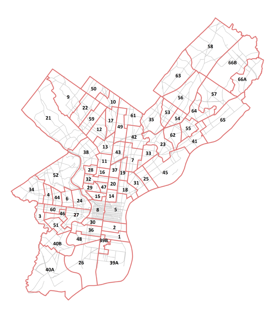
In order to help counteract that, I’m analyzing campaign finance data as it relates to local elections in Philadelphia at the ward level, specifically for the 2017 District Attorney primary election. I want to understand how money flows through the election cycle and what relationship it has with voter turnout and election results. As a Philly newbie, I had a lot to learn about ward politics, so if you are too, this is a link that explains the ward system!

Wards receive money from candidates and their political committees, the city committee, and other entities such as unions, PACs, local businesses and individuals. Candidates in particular give money to wards in order to get the ward’s endorsement and appear on their sample ballot. Thus, money flowing into wards and influencing the ward’s endorsement to voters should be transparent for the sake of democratic elections.

While Philadelphia’s campaign finance records are public, they’re tricky to analyze for several reasons. This post will detail how campaign finance records are kept, examples of how they can be analyzed using R, and a data analyst’s thoughts on how Philly campaign finance record keeping could change in the future to better accommodate accessible analysis, ultimately promoting data driven policy.

Philadelphia Campaign Finance Data 101

In Philadelphia, any entity who spends money to influence city elections is required to file a report with the Board of Ethics in Philadelphia, disclosing expenditures and contributions received. Transactions related to a state election would be filed with Harrisburg. These campaign finance reports (CFRs) are the source for “Year to Date Transaction Files” found on the phila.gov website.

While it’s great that legislation requires these campaign finance records to be filed and that they are available online for the public to download as a csv file, they have several major issues (Shout out to Bryan McHale of the Board of Ethics for helping me understand all of these):

1. There are a lot of duplicate records in the Year to Date (YTD) files because of amended reports. If you don’t remove these records any summarized totals will be greatly inflated.
2. The column which denotes whether a record is a duplicate is unreliable because it is relying on the filer to accurately check this box when they submit an amended report.
3. The entire report is hand-written, including the name of the filer and the entity. This means there are a lot of inconsistencies and spelling mistakes and summarizing on any one entity or filer is impossible without serious data cleaning work.
4. All transactions are in the YTD file, including both expenditures and contributions. So the donation of one dollar to a political campaign will be recorded multiple times as it flows from you, to the candidate, to a ward, to a get out the vote (GOTV) campaign, for example.

This project required me to create a dataset from the YTD file which showed how much money each candidate received, how much each candidate donated to each ward, and how much money each ward received from candidates and in total. In order to do so, I wrote a series of R scripts, which you can find on Azavea’s Summer of Maps Github, to account for the issues in the data outlined above and ultimately followed this path, which I’ve outlined in the rest of the blog post:

1. Understand the data structure: what columns mean and which are useful for this project
2. Filter the data to only reflect transactions that occurred in relation the 2017 primary race
3. Remove all duplicate records that occurred as a result of amended reports
4. Categorize all of the ward and candidate transactions and group and summarize by these categories
5. Visualize the results to check my work and get some preliminary findings

Year to Date File Structure and Important Columns

Every row in the dataset is a transaction representing one flow of money. The direction of the flow of money is indicated by three columns: FilerName, DocType, and EntityName.

• FilerName: Name of party filing the report. Filers can take many forms, but PACs, candidates, nonprofits, ward committees, unions, individuals, and local businesses are some prime examples.
• DocType: Schedules denote the type of transaction, either a contribution or an expenditure. For this analysis, we looked at Schedule I (contributions) and Schedule III (expenditures) transactions.
• EntityName: Receiving end of the transaction with the FilerName party.
• Cycle: Categorizes when the transaction took place; there are 14 cycles in a calendar year.
• Subdate: Submission date indicates when the campaign finance report was submitted, or when any amendments to the report were submitted.
• Transaction date: The actual date of the transaction itself.

Filtering for the 2017 Primary transactions

In order to capture transactions related to the 2017 District Attorney primary, we filtered the datasets for 2016 Cycle 7, and 2017 Cycles 1, 2, and 3. Cycle 7 covers from the end of cycle 6 in 2016 to the end of January in 2017, and cycles 4, 5, and 6 in 2017 cover activity in the general election season. To see cycle dates for the end of 2016 through the beginning of 2018, check out this link.

Removing Duplicate Records

Since the dataset includes both original campaign finance reports, as well as any reports that were re-submitted because they’d been amended, the duplicate transactions must be removed. The final submission date will generally correspond to the final report, and any of the previous submission dates will just be duplicates. To de-duplicate the data, we can create a new column that concatenates several columns: FilerName + Cycle + Year + DocType. I used a loop to cycle through every row, and for any instances of repeats in that concatenated column, I noted “keep” for the rows with the most recent submission date. I ultimately filtered for only rows that were indicated to “keep”.

This method for removing duplicates assumes that every time a filer amends a report they use the exact same spelling and capitalization for their filer name as the previous report(s) which they are amending. This assumption is the easiest to program, and given the size of the dataset, it was the only method we had time for. However, it may miss some duplicates and it is recommended that the files be sanity checked by a human before the totals are assumed to be 100% accurate.

Ward and Candidate Grouping

In order to analyze money flowing into wards, it’s necessary to group all transactions involving each ward together. However, each ward is accounted for in the YTD Transaction file a number of different ways because they are hand entered.

For example, using a text pattern search function in base R, grepl(), to find transactions related to Ward 6 illustrates these inconsistencies.

Script to search for Ward 6:

#search year to date file for ward 6 related activity 
ward_6_filername <- dat %>% filter(grepl("6th|sixth|\\b6\\b|six", FilerName, ignore.case=TRUE))

ward_6_entityname <- dat %>% filter(grepl("\\b6th\\b|sixth|\\b6\\b|six", EntityName, ignore.case=TRUE))

ward_6_names <- bind_rows(ward_6_filername, ward_6_entityname) %>% select(FilerName, Year, DocType, EntityName, Amount, Description)

The results:

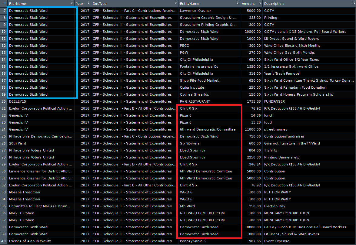
This subset of the data shows how entities file under names that are not standardized, posing obstacles for analysis. When I filter the data by FilerName for “6” “sixth” “6th” or “six”, I get the results in the blue box. And, when I search the same conditions under EntityName, the results are in the red box. In the entity column, the Democratic Sixth Ward is filed as “6th Ward Democratic Committee”, “Democratic Sixth Ward”, “6th ward Democratic Committee”, “WARD 6”, and “6TH WARD DEM EXEC COM”, along with a host of other entities that are related to the number 6 but not to a ward, like “Pizza 6” which I want to exclude.

Thus, I used these tools below in base R and dplyr in order to effectively group each ward’s transactions together.

Useful functions in R and regular expressions for cleaning unstandardized data:

• Base R:
  • grepl: matches character patterns
    • \\b \\b : acts as an anchor around a character or string . This project used it to match, for example, a 6 that’s not part of a larger number like
    • ignore.case=TRUE : argument in grepl to ignore case of character pattern when matching
    • Logic operators:
      • | = or used for positive filtering
      • & = and used for negative filtering
      • ! = not used for negative filtering
  • unique() : returns distinct occurrences of a variable
• dplyr : package in R known for manipulating data.frames
  • filter() : filter a dataframe by column value to get a subset of rows; more straightforward to use than base R’s subset()
  • select() : create a subset of variables from your data.frame
  • group_by() : group data together by variable
  • summarise() : create summary statistics of grouped data (mean, median, sum,
  • mutate() : create new columns
  • case_when() : used in tandem with mutate() to conditionally populate a new column

Filtering and negative filtering:

As shown earlier, I used grepl() to search for text in the FilerName column and EntityName column of the dataset. I want to find any transaction that is related to the number 6, for the 6th Ward.

ward_6_filername <- dat %>% filter(grepl("\\b6th\\b|sixth|\\b6\\b|six", FilerName, ignore.case=TRUE))
ward_6_entityname <- dat %>% filter(grepl("\\b6th\\b|sixth|\\b6\\b|six", EntityName, ignore.case=TRUE))

Negative/reverse filtering

I tack on a new filter statement with several !grepl statements to exclude the unrelated filing names. Note the importance of using the | operator in the positive filter and the & operator in the negative filter.

ward_6_entityname <- dat %>% filter(grepl("\\b6th\\b|sixth|\\b6\\b |six", EntityName, ignore.case=TRUE)) %>% 
  filter(!grepl("Sixsmith", EntityName, ignore.case = TRUE) & 
 !grepl("Pennsylvania 6", EntityName, ignore.case = TRUE)& 
 !grepl("Clint", EntityName, ignore.case = TRUE)& 
 !grepl("Six Workers", EntityName, ignore.case = TRUE)&                           
 !grepl("Restaurant", EntityName, ignore.case= TRUE)& 
 !grepl("Pizza", EntityName, ignore.case = TRUE))

The resulting data.frame is what we want: only EntityNames that are related to the 6th ward.

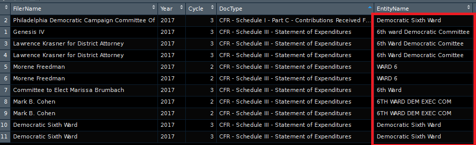
I can now combine the unique EntityNames and unique FilerNames into one vector:

w6_names <- unique(c(as.vector(unique(ward_6_filername$FilerName)),
                     as.vector(unique(ward_6_entityname$EntityName) )))

Rinse and repeat for each of the 66 wards, plus those that are split into A and B, creating vectors of all possible names wards could be referred to as.

mutate() and case_when() for assigning transactions to a ward:

Using the vectors of names, we can assign transactions to a ward, if the FilerName or EntityName matches a text value in the vector.

# create and populate "ward_ent" column for transactions that have a ward as the EntityName
dat_clean <- dat %>% mutate(ward_ent = case_when( 
  EntityName %in% w1_names ~ '1',              
  EntityName %in% w2_names ~ '2',
  EntityName %in% w3_names ~ '3'))
# ...and so on, repeating for each ward number  

# create and populate "ward_filer" column
dat_clean <- dat_clean %>% mutate(ward_filer = case_when(
  FilerName %in% w1_names ~ '1',
  FilerName %in% w2_names ~ '2',
  FilerName %in% w3_names ~ '3'))
# ...and so on, repeating for each ward number

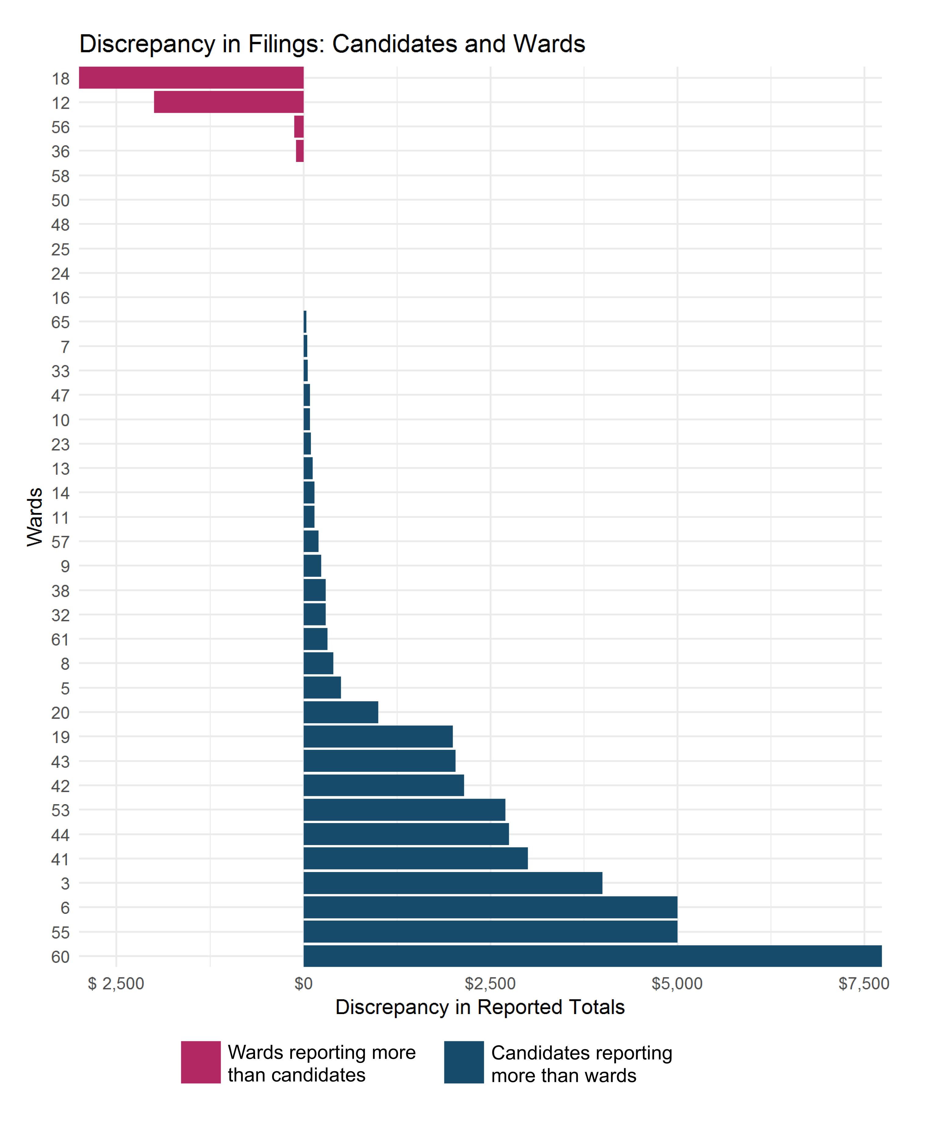
For this dataset, it’s important to retain whether the transaction involved a ward or candidate as a FilerName vs as an EntityName. A ward as a FilerName indicates that the ward submitted the report. A ward as the EntityName indicates that someone else is reporting a transaction involving that ward. It’s useful to compare what wards report receiving to what others report giving to wards and investigating discrepancies. Thus, we created columns for ward_ent as well as ward_filer.

Summarize the data with group_by and summarize():

To wrap up all of the work I put in so far in categorizing the transactions, I summarized and grouped by those different unique entities and filers. I also categorized each ward filer as either coming from Republican or Democratic committees of those wards. Because we are only looking at the Democratic DA primary, I wanted to make sure that I only included the correct committees. Committee of Seventy helped to figure out which filer belonged to which party and you can see the list they helped me compile, here on the github page.

Important notes in the code:

• Replace “NA” values with 0 so as not to break the sum function
• Use a space after “Schedule I “ in grepl to exclude a search returning Schedule III

This code first filters on DocType, to ensure this is only money wards received, indicated by Schedule I. The second line replaces NA values with 0, groups wards together, and sums the Amount column for that ward.

ward_rec_total <- dat_clean %>% filter(grepl("Schedule I ", DocType))
ward_rec_total <- ward_rec_total %>% mutate_all(funs(replace(., is.na(.), 0)))%>% group_by(ward_filer) %>% summarise(ward_rec_total = sum(Amount))
ward_rec_total <- ward_rec_total %>% filter(!ward_filer == 0) #take away row for Schedule 1 money that wasn't received by a ward 

The results of that table can ultimately be best understood with a visual, for which I used ggplot2, a package for visualizing data in R.

Using ggplot2 to visualize cleaned data:

I used ggplot2 to visualize results from this analysis, along with ggthemes, and scales. Here’s a great resource for formatting bar charts in ggplot2. In looking at the results of the data, keep in mind that this data went through a rigorous cleaning and de-duplicating process and may have errors or mistakes. Our assessment and summaries are best approximations and further digging is required before jumping to full conclusions.

Code for ggplot2 bar chart:

money_wardS_received_in_total <- 
  ggplot(dat_w_rec, aes(x = reorder(ward_filer, -dat_w_rec$ward_rec_total), y=ward_rec_total)) +   
  geom_bar(width = .85, stat="identity",position="identity", fill = "#FFA07A") +  
  scale_y_continuous(labels = scales::dollar, expand = c(0,0)) + 
  labs(y="Amount Received", title = "Money received by wards in the 2017 Primary", x="Wards") +
  theme_minimal() +
  theme(axis.text.x=element_text(size = 4.8, color = "black", angle = 65)) + 
  geom_hline(aes(yintercept = avg), colour="#5A594E", linetype="dashed") + 
  geom_text(aes(50, avg, label = "Average Amount", vjust = 1.5), size = 3, colour="#5A594E") + 
    geom_text(aes(label = ward_filer, vjust = 2), color="black", size = 1.6)

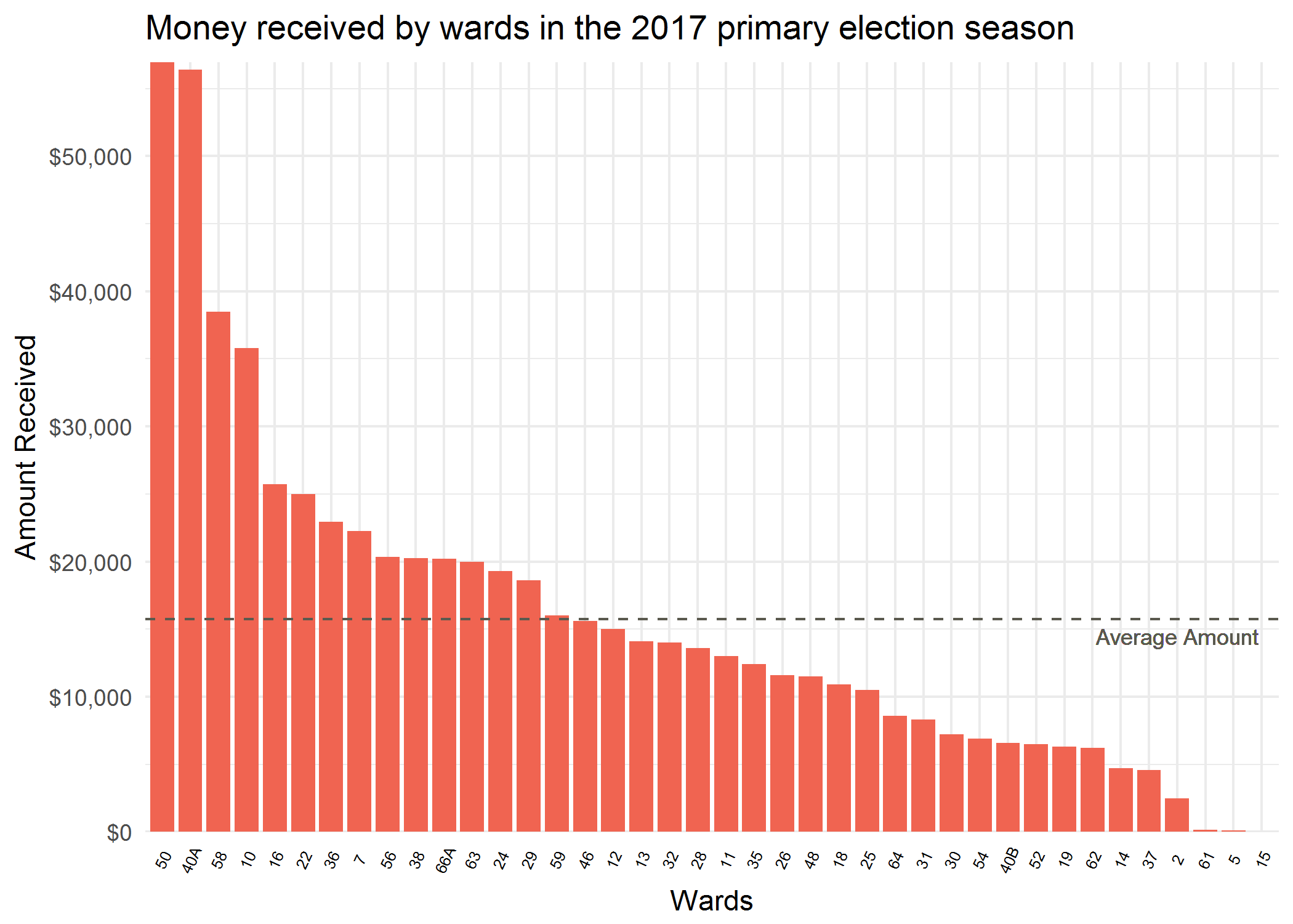
The resulting bar chart shows a few key pieces of information. The spread of money flowing into wards during the primary season ranges from $0 to $55,000, with an average amount of money flowing into wards at around $16,000. The data used is ward-reported and only visualizes contributions to the ward that include a monetary amount (in-kind contributions are not visualized).

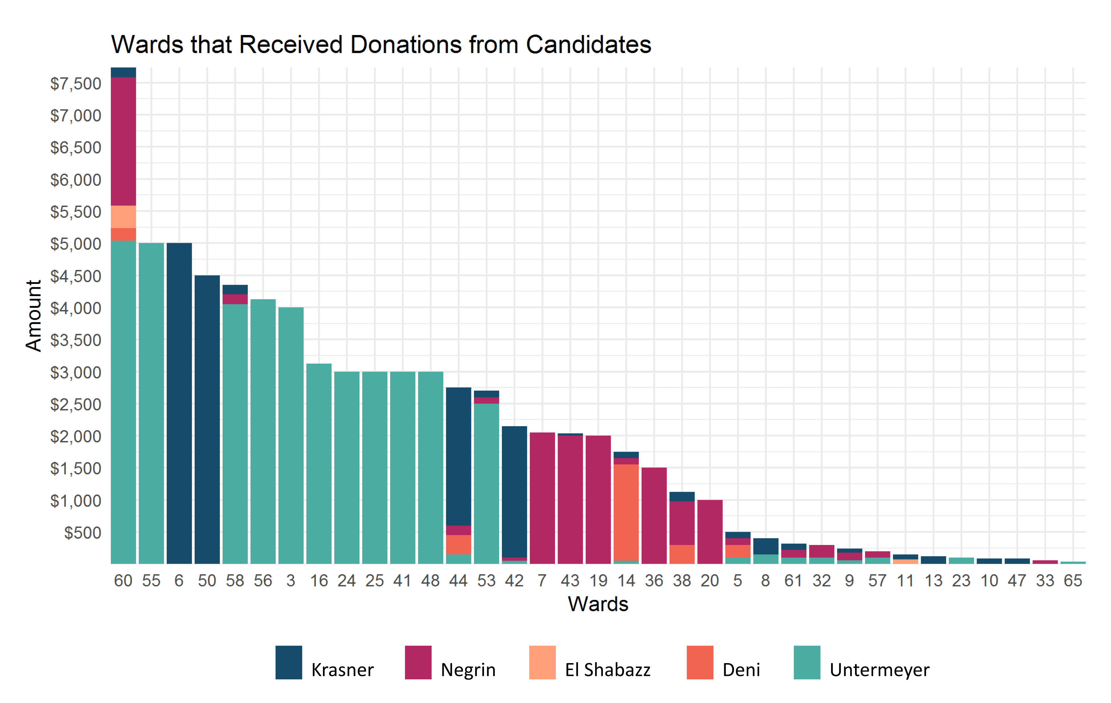
A few more barcharts I was able to produce using ggplot2 show how much money each ward received from each candidate and the discrepancy in filing between what the wards reported receiving and what the candidates reported giving.

Thoughts on Promoting Analysis-ready Campaign Finance Records

Philadelphia has made great strides in advancing democracy through campaign finance regulations, and publicly available campaign finance records are crucial for transparent elections. However, there’s a learning curve to the Year to Date Transaction files, and in tandem with the data being un-standardized, these obstacles stand in the way of public engagement with local politics.

As a data analyst who’s become familiar with this dataset, I can offer thoughts on how the records could change in the future to accommodate more streamlined analysis.

Primarily, I suggest standardization in the form of identification codes for each political entity (ward committee, ward leader, candidate, PAC, etc.). Codes would be available online for easy look-up, and any activity related to that entity would be easily searchable. Policy makers and citizens alike could query a candidate’s spending record, or how much money a ward is receiving from a candidate without the prerequisite of a working knowledge in a statistical programming language. It would also be useful for in-kind contributions to be filed with an estimated dollar amount for the worth of the contribution, and thus lend themselves to inclusion in monetary analysis.

Additionally, the clarity of the reports could be greatly improved by including only final versions of the campaign finance reports in the dataset.

In short, informed citizens are the foundation of a healthy democracy. Regulated campaign finance is important for transparent elections, but enforcing and updating regulations can be streamlined with forward-thinking and intentionally designed datasets. In the case of Philadelphia campaign finance records, publicly available datasets don’t equate to accessible datasets in terms of citizen engagement or analysis.

Similar to a lot of Azavea’s work, the scripts I used for this project are available under an open source license. If you would like to replicate my work, check out the scripts on Azavea’s Summer of Maps Github.