This blog is accompanied by a Colab notebook which provides an in-depth look at how Raster Vision works and allows you to run each experiment discussed in this post yourself.

Change detection is the computer-vision equivalent of the spot-the-difference game. Given two images, the model must detect all the points at which they differ. In the context of remote sensing, these images are usually satellite or aerial images of the same geographical location at two different points in time.

Change detection has been an active research area for a long time and the literature is rich with algorithms that perform the task automatically, ranging from basic image processing techniques to present-day deep neural networks. And these algorithms have a wide range of applications including detection of deforestation, damaged buildings in the wake of disasters, and changes in urban land use. See, for example, [1] for an up-to-date review of change detection techniques.

A broad way to categorize change detection techniques is by how they model change. The direct classification approach models the change itself. In the supervised machine learning context, this requires annotations in the form of “change masks”; these masks might either be binary (change / no-change) or more specific (with classes like “forest-to-land”, “land-to-water”, etc.). The post-classification approach, on the other hand, models the underlying features (e.g. tree cover) in an image and then compares those features from both images to see what has changed. For this, one needs annotations for these features rather than for the changes. When working at the pixel-level, both approaches amount to semantic segmentation.

This blog will explore the direct classification approach to change detection using our open-source geospatial deep learning framework, Raster Vision, and the publicly available Onera Satellite Change Detection (OSCD) dataset. Raster Vision allows us to easily tackle the peculiarities of this dataset and set up a semantic segmentation training pipeline that can quickly produce a decent model.

Using the OSCD dataset

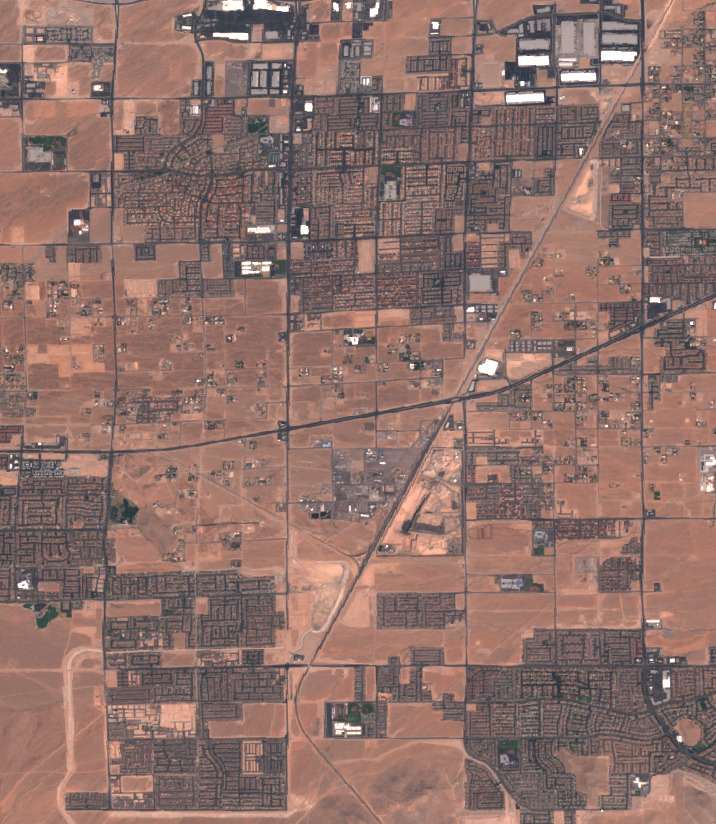
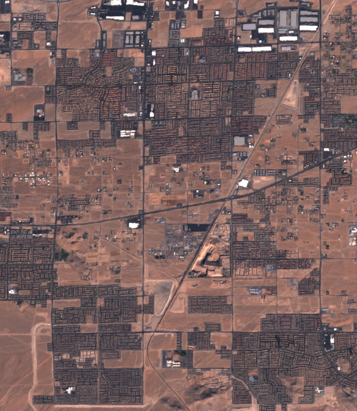
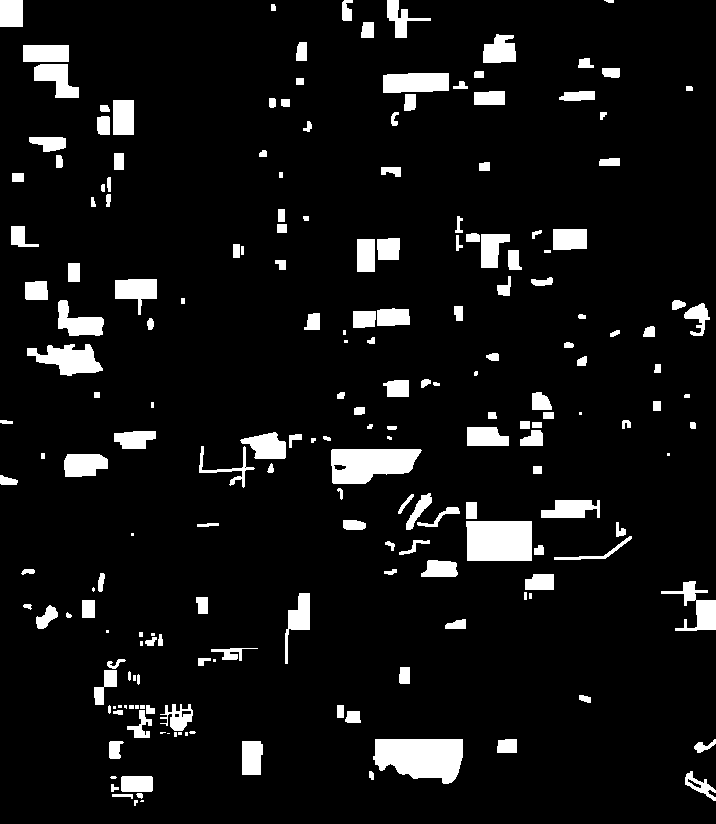
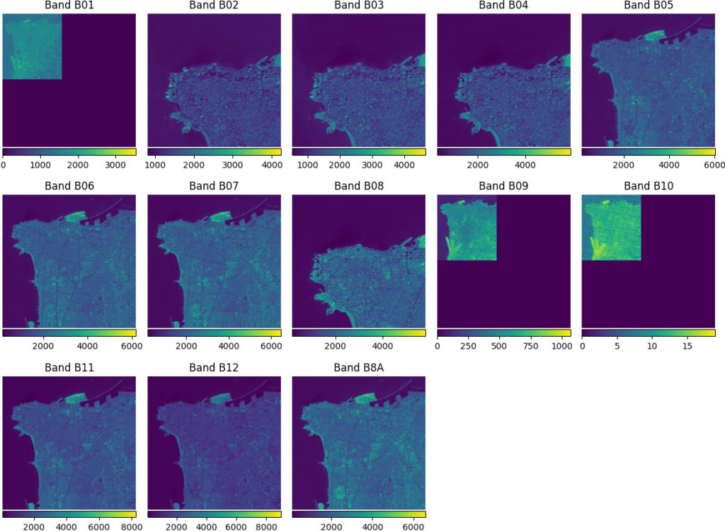
The Onera Satellite Change Detection dataset [2] is a dataset comprising 24 co-registered pairs of 13-band multi-spectral Sentinel-2 satellite images taken between 2015 and 2018. For each pair of images, there are corresponding change detection annotations provided in the form of pixel-level labels for change and no change. Each image pair is from a different city; some examples are: Beirut, Las Vegas, Mumbai, Paris, and Valencia.

14 of the 24 image-pairs are for training, while the remaining 10 make up the hold-out test set.

Data challenges

The dataset presents some challenges that must be overcome before we can use it for training a model:

• All the bands in each image are separate files that must be stacked together to form the full multispectral image.
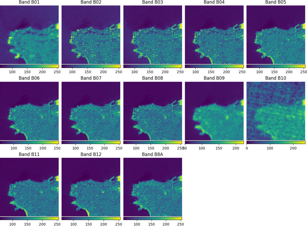
• Stacking the bands together is not trivial as they do not all share the same resolution. So a given window of size, say, 400×400 pixels does not correspond to the same geographical area in each band as can be seen in the image below.

Machine learning challenges

Apart from the data challenges, there are also some challenges from a machine learning perspective. These do not hinder use of the data but likely make training a good model harder:

• The distribution of pixel intensity values differs significantly among bands. This could slow down training because the weights in the model’s first convolutional layer will need to be adjusted to handle the different scales of values in each band.
• The dataset is relatively small. There are only 14 training image-pairs and all of them have too low a resolution to be able to generate a large number of training chips.
• Class imbalance. No-change pixels greatly outnumber change pixels.

Raster Vision’s solutions

Luckily, Raster Vision has potential solutions for all of these:

• The challenge of extracting bands from different files and stacking them so that they are geographically aligned is easily solved by using the MultiRasterSource abstraction which performs the alignment automatically. 
• Pixel distributions of bands can be homogenized using the StatsTransformer which normalizes each band’s pixel values to the 0-255 range while also clipping outlier values. (These are converted to 0-1 before being passed to the model.)
• The smallness of the dataset can be somewhat addressed by using data augmentation. One simple way to augment the training data would be to also use the existing image-pairs with their orders reversed. Raster Vision accepts arbitrary albumentations transforms for data augmentation, so we can define a custom albumentations transform to do this.
• To address the class imbalance, Raster Vision allows specifying weights for each class that will be used to weight contribution of each class to the loss. We can use this to assign a larger weight to the change class.

Machine learning experiments

Using Raster Vision, we split the 14 training scenes into training and validation sets of 10 and 4 scenes respectively and experimented with the following:

• Training with and without band normalization.
• Using a weighted loss to offset the class imbalance.
• Randomly swapping the order of the two images as a form of data augmentation.

Each experiment used a Panoptic FPN [3] model with a ResNet-50 [4] backbone that was trained for 10 epochs with an Adam optimizer with an initial learning rate of 0.01 and a one-cycle schedule, and a batch size of 16.

The results of these experiments on the validation set are summarized in the table below.

Change:No-change Loss Weight Ratio	Image Swap Augmentation	Normalization	Change Recall	Change Precision	Change F1 Score
1:1			0.286	0.583	0.384
10:1	X		0.291	0.668	0.405
10:1	X	X	0.398	0.609	0.482
20:1	X	X	0.751	0.229	0.351

We see that the best F1-score is achieved by the model in the third row. Empirically, the loss weighting, data augmentation, and band normalization seem to help, but we will need to run each experiment multiple times or do cross validation to give these observations statistical backing.

Evaluating on the test set

Raster Vision’s predict command allows us to make predictions on each scene in the test set. This prediction happens in a sliding-window fashion and we can optionally reduce the stride to ensure that each pixel gets predicted multiple times and the results are averaged — this functions as a kind of test time augmentation.

With the predictions in place, Raster Vision’s eval command can be run to compare these with the ground truth to automatically compute performance metrics and stores them in a JSON file.

Running predict and eval for the best model from the table above for the held-out test set of 10 scenes, we get the results shown in the table below.

The table also compares these results with other published results on this dataset. [2] is the paper that introduced this dataset and [3] is a follow-up paper by the same authors that introduces new specialized architectures, FC-Siam-conc and FC-Siam-diff, for change detection. We can see that our model, despite not being especially designed for change detection, outperforms the models from [2] and is roughly on par with the FC-Siam-conc architecture from [3].

Model	Change Recall	Change Precision	Change F1 Score
Panoptic FPN (Ours)	0.676	0.411	0.511
Siam. [2]	0.856	0.242	0.377
EF [2]	0.847	0.284	0.485
FC-Siam-conc [3]	0.652	0.424	0.514
FC-Siam-diff [3]	0.580	0.578	0.579

Visualizing the model’s predictions

While numbers are fine for comparing experiments, they do not give us an intuitive sense of what the model is actually doing. For this, we need to look at the actual predictions.

The following GIFs (you might need to play them manually if auto-play doesn’t work) show some of the outputs produced by the model on images from the validation and test sets. The areas where the model detected change are outlined in red. We can see that the model does a pretty good job of detecting the most prominent changes while ignoring irrelevant changes like slight changes in color.

Conclusion

As imaging satellites continue to grow in both number and capability, applications that involve continuous Earth monitoring will become increasingly common. Keeping track of, for example, deforestation or melting glaciers, is also particularly relevant from a climate change perspective, which continues to be an important focus for us as a company.

Timely and accurate change detection forms a crucial part of such monitoring efforts. Given the sheer amount of data, much of this analysis must necessarily be performed by computer-vision models rather than humans. Free and open-source tools like Raster Vision ensure that the ability to train such state-of-the-art models is available to everyone.

References

[1] Shi, Wenzhong, Min Zhang, Rui Zhang, Shanxiong Chen, and Zhao Zhan. “Change detection based on artificial intelligence: State-of-the-art and challenges.” Remote Sensing 12, no. 10 (2020): 1688.

[2] Daudt, R.C., Le Saux, B., Boulch, A. and Gousseau, Y., 2018, July. Urban Change Detection for Multispectral Earth Observation Using Convolutional Neural Networks. In IEEE International Geoscience and Remote Sensing Symposium (IGARSS) 2018 (pp. 2115-2118). IEEE.

[3] Kirillov, Alexander, Ross Girshick, Kaiming He, and Piotr Dollár. “Panoptic feature pyramid networks.” In Proceedings of the IEEE/CVF Conference on Computer Vision and Pattern Recognition, pp. 6399-6408. 2019.

[4] He, Kaiming, Xiangyu Zhang, Shaoqing Ren, and Jian Sun. “Deep residual learning for image recognition.” In Proceedings of the IEEE conference on computer vision and pattern recognition, pp. 770-778. 2016.