As we near the administration of the Bipartisan Infrastructure Investment and Jobs Act, decision-makers across the country are likely thinking of how to secure and utilize this funding. Eliminating lead service lines, expanding broadband internet access, and repairing roads and bridges are of major concern in many communities across the country.

Looking ahead, it likely won’t be the last time we experience similar funding as the effects of climate change will only increase the need for infrastructure improvements over time. As communities brace for the inevitable changes that lie ahead, it’s imperative that we create and use tools like the Rural Capacity Index to highlight the disparities that exist between communities that are able to apply for this funding and those that are less resourced and lack the capacity to access this capital. Accessing federal funds requires experienced staff that have the time to write the proposals, the resources to build and design the projects that need funding, and the ability to maintain these projects long term. Communities that lack the skill and labor to apply for these funds tend to need these resources the most and are often several steps behind larger cities that have fewer roadblocks when applying.

The Technical Process/Partnering with Headwaters Economics

In an attempt to address the disparity in access to funding resources, we partnered with Headwaters Economics to develop and normalize a set of metrics to create an overall score for each county in the U.S. Software Engineer Adeel Hassan and Senior GIS Analyst Daniel McGlone identified the metrics used to create the index with Headwaters Economics, normalized the final variables that were selected, and calculated the index for each county, county subdivision, and census-designated place in the U.S. Let’s dig into this process, look at how important data decisions were made, and discuss some of the solutions to problems that arose like variable transformations and missing data.

Choosing the Right Variables to Calculate the Index

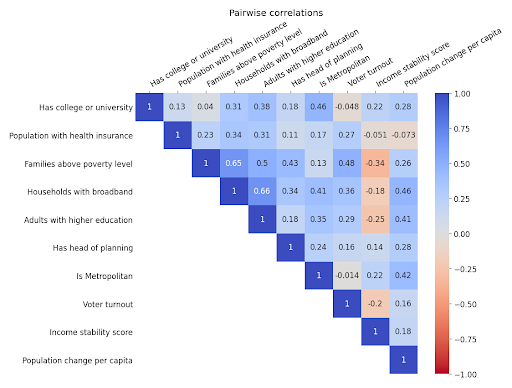
First, we sat down with Headwaters Economics and came up with a preliminary list of variables to be considered when calculating the index formula. We then took this list and identified reliable sources to acquire this data. With input from Headwaters Economics, we pared down the preliminary list to the most relevant metrics. Variables were eliminated if we could not find a trustworthy data source, the data was incomplete, and if variables were highly correlated with other options on the list which would ultimately make them redundant as they’d be measuring the same concept. We then acquired all of the data from sources such as the U.S. Census Bureau, Power Almanac, the Bureau of Economic Analysis, and others. Here is the final list of variables used to calculate the index:

• Metropolitan / is_urban  (per the CDC: Metropolitan counties: contain the entire population of the largest principal city of the MSA, or 2) are completely contained within the largest principal city of the MSA, or 3) contain at least 250,000 residents of any principal city in the MSA)
• Has head of planning / has_head_of_planning 
• Has college or university / has_university 
• Adults with higher education / pct_bachelor_or_higher 
• Families above poverty level / pct_families_not_in_poverty 
• Households with broadband / pct_broadband 
• Population with health insurance / pct_insured 
• Voter turnout / pct_voter_turnout 
• Income stability score / inv_income_stdev
• Population change / population_change_per_capita

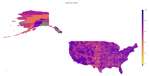
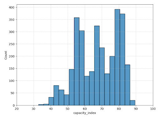
In order to analyze and visualize the capacity of each county in the U.S., the variables collected must be joined to spatial data. Once the data was gathered, the next step was to match this information to its relevant county. In some cases, this was easily accomplished using the county’s FIPS code; in other cases, we had to resort to a spatial join. After performing the join, we normalized the data in Python in order to calculate the final index. Each variable was transformed so that the value was between 0 and 100. We then calculated the Rural Capacity Index for each county as the unweighted mean of all the corresponding normalized variables. Communities on the Pacific Coast and in the Northeast ranked the highest, while counties in the Midwest and on the Gulf Coast ranked the lowest.

Limitations and Issues We Addressed

Working with data and creating indices is never a flawless process. Especially when bringing a spatial component to information, there will usually be edge cases that need to be addressed manually.

Variable Transformations

While some of the variables were already in the right form to be fed into the index formula, others needed some massaging. For example, we transformed the original lower-is-better income standard deviation variable to better match our higher-is-better capacity index. Since we want to give a higher score to lower-income standard deviations, we had to invert or flip these values. This task was made trickier by the fact that these values are distributed across several orders of magnitude (ranging from the hundreds to the tens of thousands). After assessing three different options to address this issue, we found the best solution was to invert after applying a log transformation. More specifically:

Missing Data

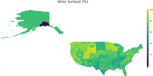
Some variables had data missing for a significant number of counties/communities. For example, the voter turnout data was missing for all counties in the states of Alaska, Florida, Kansas, North Dakota, South Dakota, and Tennessee. For these, we used the state-level voter turnouts as a substitute.

No indicator or index will ever be perfect. The variables selected for this index prioritized the assessment of rural communities over metropolitan areas, as the latter historically have more resources to address infrastructure-related issues. This prioritization means that Wayne County, MI (home to Detroit), an area that has experienced decades of disinvestment and is desperate for resources, scores relatively high despite its glaring needs. Detroit’s capacity index score is lower than most nearby urban areas (Milwaukee, Chicago, Cleveland, etc.), but is higher than most rural areas.

What’s Next?

We partnered with Headwaters Economics to develop and normalize a set of metrics to create an overall capacity score for each county in the US. We leaned on them for their expertise in developing the methodology while we provided our geospatial and technical expertise in selecting data sources, preparing data, and presenting data spatially. We are always excited by the work of Headwaters Economics and jumped at the opportunity to co-develop the Rural Capacity Index.

The Rural Capacity Index is a tool that sheds light on areas in the U.S. that may need more attention when it comes time to apply for funding. This index is a starting point for addressing how funding is dispersed and how low-capacity communities can more effectively advocate for direct funding (without having to compete with communities with more capacity to apply). These visuals could also be overlaid with other climate data that indicate areas that are prone to wildfires, drought, and other extreme weather. Headwaters Economics works directly with communities and suggests tools like the Rural Capacity Index to advocate for resources. They also argue that the Rural Capacity Index can be used by federal and state agencies to more deliberately invest in communities that would otherwise be left behind.

Interested in working together to build compelling visualizations and tell a story? Contact us now – we’d love to chat.