
This summer, Adeel joined the team as an Azavea Open Source Fellow to work on Raster Vision, our open-source framework for deep learning on satellite and aerial imagery. The Azavea Open Source Fellowship program is a 12-week professional training fellowship that matches software engineering fellows with open source projects at Azavea.
Introduction
Satellite imagery is often multi-spectral i.e comprising other bands besides the usual Red, Green, and Blue (RGB). These may be either other electromagnetic bands, such as Infra-red or Ultraviolet, or something very different like Elevation.
While using these images for Machine Learning on any Computer Vision task, we would ideally like to make use of all available bands, since each of them might carry unique information that could potentially improve model performance. Unfortunately, in practice, we usually find ourselves sticking with either just RGB or some other combination of 3 bands.
Why? Because these days, it is standard practice to use Transfer Learning to make use of pre-trained models instead of training a brand new model from scratch. These are models that have been pre-trained on millions of ImageNet images; they can be relatively quickly fine-tuned to adapt to any new dataset, and generally outperform models trained from scratch on the task-specific dataset. But the images these models have been trained on are RGB images, and so, if you want to take advantage of them, you must restrict yourself to 3 channels. Interestingly, these models even outperform from-scratch models trained on more than 3 bands.
But what if we could avoid having to make this tradeoff? What if we could make use of pre-trained RGB models as well as additional bands? To be clear, this would go beyond ordinary Transfer Learning, where you fine-tune on a new dataset; here, we would not only be fine-tuning on a new dataset but also simultaneously training the model to take in new input features (the new channels).
So how do we go about this? We need to preserve as much of the pre-trained model weights as possible, yet still, somehow modify the network such that it can ‘see’ the additional bands.
One possibility is to expand the convolution filters in the first layer so that they have more than 3 channels. The RGB channels of these filters will be initialized with the pre-trained weights, while the new channels will start off from scratch and will need to be learned (Figure 1).
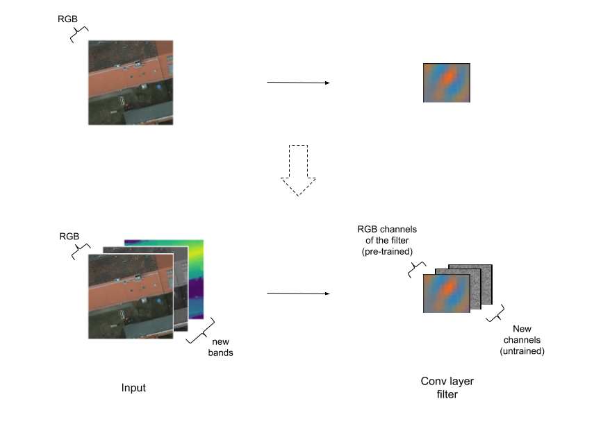
Figure 1: Extending convolutional filters by adding extra channels.
Mathematically, this is equivalent to having 2 convolutional layers in parallel, one that acts on RGB channels, and one that acts on the other channels, and then adding their outputs (Figure 2).
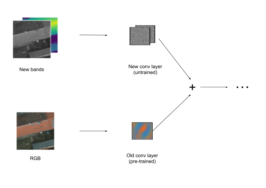
Figure 2: Adding extra channels is equivalent to adding a parallel convolutional layer and adding the results.
Seen this way, a couple of ways to generalize the concept of the “parallel layer” become apparent (Figure 3). For instance, we may ask: is there a way to merge the output of the two layers other than simple addition? We may also ask if the best place to do this merging is after the first convolutional layer or is there perhaps some other point deeper within the network that would work better. If we choose to merge at a deeper point we will need to replicate all the layers up to that point.
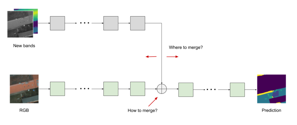
Figure 3: Considerations when adding a parallel layer: where and how to merge.
So, the 2 major questions we attempted to answer with this project are:
- Does including additional bands help at all?
- Which particular technique of including additional bands works best?
Approach and experiments
Problem and dataset
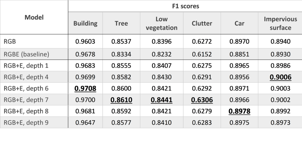
For most of our experiments, we worked with the task of multi-class Semantic Segmentation (Figure 5) on the ISPRS Potsdam dataset (Figure 4). The dataset consists of satellite images of the city of Potsdam and has 6 classes of objects: buildings, trees, low vegetation, clutter, cars, and impervious surfaces. Each image has 5 bands: R, G, B, IR, and Elevation. We restricted ourselves to adding only the Elevation band to the RGB model.
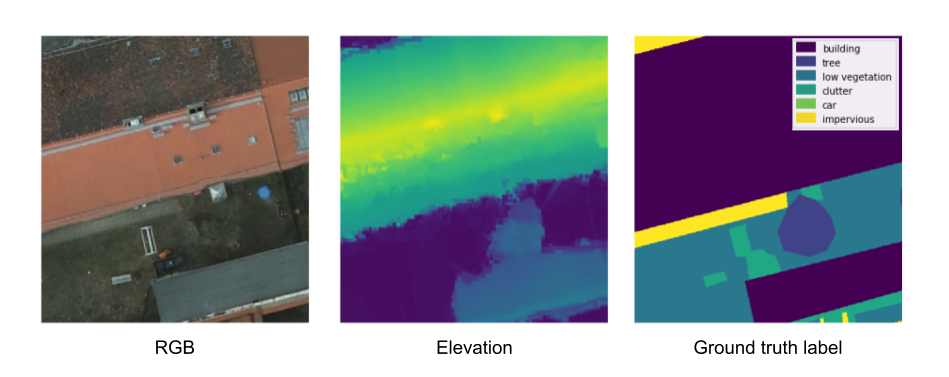
Figure 4: Example image from the Potsdam dataset. Left: RGB image. Middle: The elevation channel for the same image. Right: The corresponding Ground Truth labels.
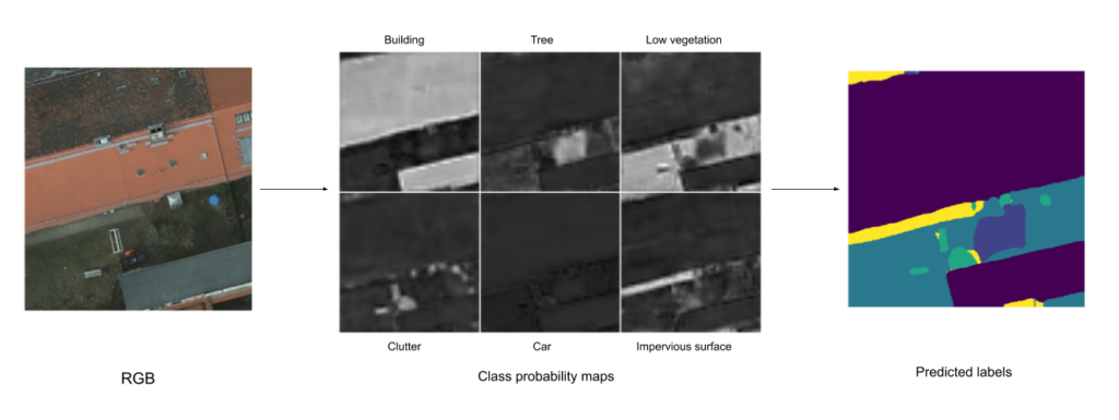
Figure 5: How semantic segmentation models work: an input image is fed into the model, the model outputs probability maps for each class, a final prediction is generated by searching for the max probability across all class probability maps for each pixel.
Models
All the experiments discussed here were done using the PyTorch TorchVision implementation of the DeepLabV3 (also see here) network with a ResNet-101 backbone.
Experiments
How to merge?
We experimented with 2 different methods of merging the parallel layers:
- Simple addition (Figure 6)
- Concatenation followed by a 1×1 convolution layer to project the output to a size compatible with the next layer (Figure 7)
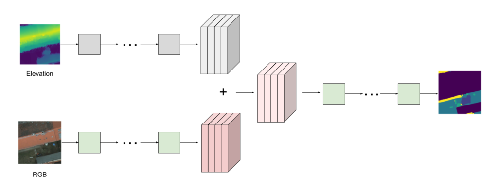
Figure 6: Merging parallel layers by adding their outputs. The outputs must be the same size.
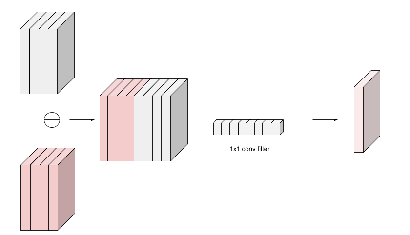
Figure 7: Merging parallel layers by concatenating their outputs along the channel dimension and then projecting to the desired number of channels by using a 1×1 convolution layer.
Where to merge?
We experimented with merging at 6 different points within the DeepLab network: 4 points within the ResNet backbone, 1 point immediately after the backbone, and 1 after the ASPP (Atrous Spatial Pyramid Pooling) layer (Figure 8).
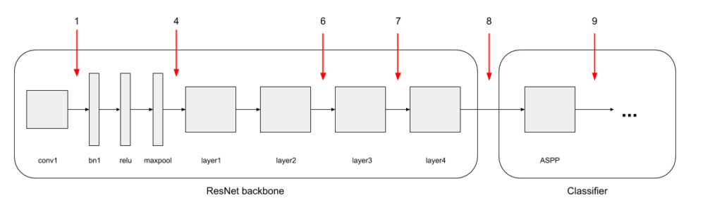
Figure 8: Overview of the DeepLab architecture. Merge points shown in Red.
Training procedure
The training procedure involved:
- Fine-tuning a pre-trained DeepLab model on RGB images – the RGB model
- Starting from a pre-trained DeepLab model, replacing its first conv layer with a single channel conv layer, and training it on just the Elevation band – the E model
- Combining the two by taking some initial layers from the E model and merging them into the RGB model – the RGB+E model
- Training the RGB+E model end-to-end
Baseline
Besides comparing with the RGB model, we also compared with a baseline RGBE model. This is a model that was initialized with a pretrained ResNet backbone, and then had its first (3-channel by default) conv layer replaced with a randomly initialized 4-channel conv layer. It was then trained end-to-end on RGBE data.
Results and analysis
So what answers did we come up with for our 2 questions?
Does including additional bands help at all?
Yes! A comparison of F1-scores shows that all our RGB+E models outperform the RGB-only model across almost all classes. We also see that the baseline RGBE model performs even worse than the RGB-only model for most classes, highlighting the importance of retaining the pretrained RGB filters.
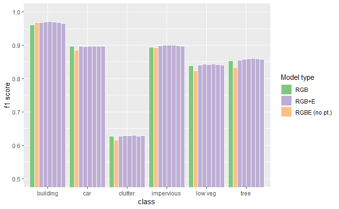
Figure 9: Performance comparison between an RGB only model, the RGBE baseline model, and several RGB+E models (with different merge depths). Results averaged over multiple runs.
While comparing F1-scores is nice and all, it would be great if we could see an example of an image where the addition of elevation leads to a clearly better output. Annoyingly, finding such examples is hard because the RGB model is still pretty good and doesn’t make a lot of glaring mistakes.
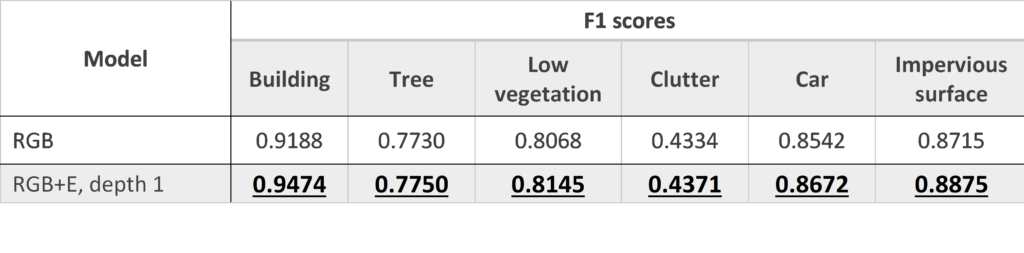
To address this, we train a new pair of RGB and RGB+E models, but this time on only 20% of the training set. The idea is to make the RGB part of the model worse so that it will have to rely more often and more strongly on the Elevation info. Having done this, we find larger improvements for some classes, especially the building class.
We also find good visual examples, such as this one:
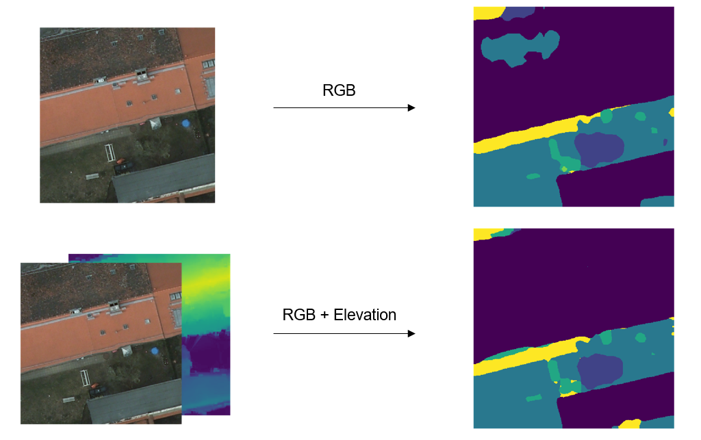
Figure 10: Top: Output of the RGB-only model given the RGB image as input. Bottom: Output of the RGB+E model given the RGBE image as input.
Here we can see that the RGB model misclassifies part of a building as “low vegetation”, but the RGE+E model, presumably making use of the Elevation info, does not.
But is the improvement really due to the model making use of elevation? One way to test this is to manipulate the elevation values in the above example and see if that affects the model’s outputs.
Let’s say we set the elevation value of all pixels to 0 (zero). This means that we are telling the model that everything in the image is on the ground. If the model has really developed a reasonable understanding of “elevation”, we expect that this will confuse the model.
And it does:
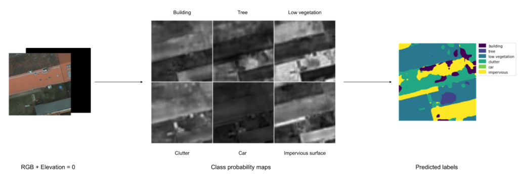
Figure 11: Output of the RGB+E model given an image with all elevation values (deviously) set to 0.
We see that the model is now less sure about its building and tree predictions and the probabilities of ground-based classes like “low vegetation” and “impervious surface” have gone up.
How about if we set all elevation values to 1 (the maximum value) instead? Is the model output still affected as expected?
Indeed it is:
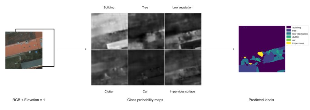
Figure 12: Output of the RGB+E model given an image with all elevation values (deviously) set to 1.
Here we see that the model is more confident about its building predictions – in fact, it now seems to suspect buildings everywhere! We also notice that a new tree has shown up! It seems the decision process there was “green area + high elevation = tree”, which is fairly good reasoning. Also, the probabilities of ground-based classes have gone down.
From this, we conclude that the model has learned to understand elevation.
Which particular technique of including additional bands works best?
How to merge?
We did not find any significant performance differences between addition and the 1×1 convolution method in our preliminary experiments, and therefore, chose to stick with the simpler of the two methods i.e. addition for the rest of our experiments.
Where to merge?
Comparing the performance of models with different merge depths, there does seem to be a slight pattern apparent for at least buildings, low vegetation, and trees, where the highest performance is achieved at a depth somewhere in the middle of the ResNet backbone. While not straightforwardly interpretable, and possibly not statistically significant, this is something that might be worth investigating further.
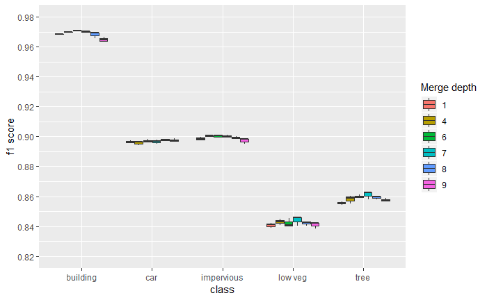
Figure 13: Boxplot comparing the performance for the RGB+E model for various merge depths.
Conclusions
We have shown that we can teach a model to take advantage of extra channels without discarding the original RGB pre-training, resulting in significant performance improvement over the RGB-only model.
We now have a recipe for readily incorporating additional bands into any neural network for any Computer Vision problem, at least as far as merging after the first conv layer is concerned. For greater depths, while we know how to handle sequential models like DeepLab, it is not trivial to carry out this procedure for networks with skip connections, such as UNet.
Future work
It would be interesting to try this out on other datasets and see if we can replicate the promising results seen here. In particular, we would like to try out this approach on RGB-D datasets and see how it compares to other approaches.
We are also working on coming up with a way to theoretically estimate the usefulness of adding new channels. Since this is essentially the same as adding new input features, a lot of the theory around information gain and mutual information should apply here.