
Aerial and satellite imagery gives us the unique ability to look down and see the earth from above. It is being used to measure deforestation, map damaged areas after natural disasters, spot looted archaeological sites, and has many more current and untapped use cases. At Azavea, we understand the potential impact that imagery can have on our understanding of the world. We also understand that the enormous and ever-growing amount of imagery presents a significant challenge: how can we derive value and insights from all of this data? There are not enough people to look at all of the images all of the time. That’s why we are building tools and techniques to allow technology to see what we cannot.
One such tool that we are currently developing at Azavea is Raster Vision. This project encapsulates a workflow for using deep learning to understand and analyze geospatial imagery. The functionality in Raster Vision will be made accessible through Raster Foundry, Azavea’s product to help users gain insight from geospatial data quickly, repeatably, and at any scale. Like Raster Foundry and much of the software developed at Azavea, Raster Vision is open source. It is released under an Apache 2.0 license and developed in the open on GitHub. This allows anyone to use and contribute to the project. It can also provide a starting point for others getting up to speed in this area.
Raster Vision began with our work on performing semantic segmentation on aerial imagery provided by ISPRS. In this post, we’ll discuss our approach to analyzing this dataset. We’ll describe the main model architecture we used, how we implemented it in Keras and Tensorflow, and talk about various experiments we ran using the ISPRS data. We then discuss how we used other open source tools built at Azavea to visualize our results, show some analysis of deep learning inside interactive web mapping tools, and conclude with directions for future work.
Semantic Segmentation and the ISPRS contest
The goal of semantic segmentation is to automatically label each pixel in an image with its semantic category. The ISPRS contest challenged us to create a semantic segmentation of high resolution aerial imagery covering parts of Potsdam, Germany. As part of the challenge, ISPRS released a benchmark dataset containing 5cm resolution imagery having five channels including red, green, blue, IR and elevation. Part of the dataset had been labeled by hand with six labels including impervious, buildings, low vegetation, trees, cars, and clutter, which accounts for anything not in the previous categories. The dataset contains 38 6000×6000 patches and is divided into a development set, where the labels are provided and used for training models, and a test set, where the labels are hidden and are used by the contest organizer to test the performance of trained models.
Deep learning has been successfully applied to a wide range of computer vision problems, and is a good fit for semantic segmentation tasks such as this. We tried a number of different deep neural network architectures to infer the labels of the test set. To construct and train the neural networks, we used the popular Keras and Tensorflow libraries. Our code was designed following the principles in the blog post “Patterns for Research in Machine Learning”, and is intended to make it easy to try different datasets, data generators, model architectures, hyperparameter settings, and evaluation methods.
Fully Convolutional Networks
There has been a lot of research on using convolutional neural networks for image recognition, the task of predicting a single label for an entire image. Most recognition models consist of a series of convolutional and pooling layers followed by a fully-connected layer that maps from a 3D array to a 1D array of probabilities.

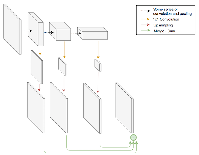
The Fully Convolutional Network (FCN) approach to semantic segmentation works by adapting and repurposing recognition models so that they are suitable for segmentation. One challenge in upgrading recognition models to segmentation models is that they have 1D output (a probability for each label), whereas segmentation models have 3D output (a probability vector for each pixel). By removing the final fully-connected layer, we can obtain a “fully convolutional” model that has 3D output. However, the final convolutional layer will still have too many channels (typically > 512) and too low a spatial resolution (typically 8×8). To get the desired output shape, we can use a 1×1 convolutional layer which squashes the number of channels down to the number of labels, and then use bilinear interpolation to upsample back to the spatial resolution of the input image.
Despite having the correct resolution, the output will be spatially coarse, since it is the result of upsampling, and the model will have trouble segmenting small objects such as cars. To solve this problem, we can incorporate information from earlier, finer-grained layers into the output of the model. We can do this by performing convolution and upsampling on the final 32×32, 16×16, and 8×8 layers of the recognition model, and then summing these together.
The FCN was originally proposed as an adaptation of the VGG recognition model, but can be used to adapt newer recognition models such as ResNets, which we used in our experiments. One advantage of the FCN over other architectures is that it is easy to initialize the bulk of the model using weights that were obtained from training on a large object recognition dataset such as ImageNet. This is often helpful when the size of the training set is small relative to the complexity of the model.
Here is a code snippet that shows how to adapt a ResNet into an FCN using Keras. It is impressive how concisely this can be expressed, and how closely the code matches the graphical representation shown above.
# The number of output labels
nb_labels = 6

# The dimensions of the input images
nb_rows = 256
nb_cols = 256

# A ResNet model with weights from training on ImageNet. This will
# be adapted via graph surgery into an FCN.
base_model = ResNet50(
    include_top=False, weights='imagenet', input_tensor=input_tensor)

# Get final 32x32, 16x16, and 8x8 layers in the original
# ResNet by that layers's name.
x32 = base_model.get_layer('final_32').output
x16 = base_model.get_layer('final_16').output
x8 = base_model.get_layer('final_x8').output

# Compress each skip connection so it has nb_labels channels.
c32 = Convolution2D(nb_labels, (1, 1))(x32)
c16 = Convolution2D(nb_labels, (1, 1))(x16)
c8 = Convolution2D(nb_labels, (1, 1))(x8)

# Resize each compressed skip connection using bilinear interpolation.
# This operation isn't built into Keras, so we use a LambdaLayer
# which allows calling a Tensorflow operation.
def resize_bilinear(images):
    return tf.image.resize_bilinear(images, [nb_rows, nb_cols])

r32 = Lambda(resize_bilinear)(c32)
r16 = Lambda(resize_bilinear)(c16)
r8 = Lambda(resize_bilinear)(c8)

# Merge the three layers together using summation.
m = Add()([r32, r16, r8])

# Add softmax layer to get probabilities as output. We need to reshape
# and then un-reshape because Keras expects input to softmax to
# be 2D.
x = Reshape((nb_rows * nb_cols, nb_labels))(m)
x = Activation('softmax')(x)
x = Reshape((nb_rows, nb_cols, nb_labels))(x)

fcn_model = Model(input=input_tensor, output=x)
Experiments
We ran many experiments, and the following are some of the most interesting. Each experiment was specified by a JSON file stored in version control, which helped keep us organized and makes it easier to replicate our results.
ResNet50 FCN
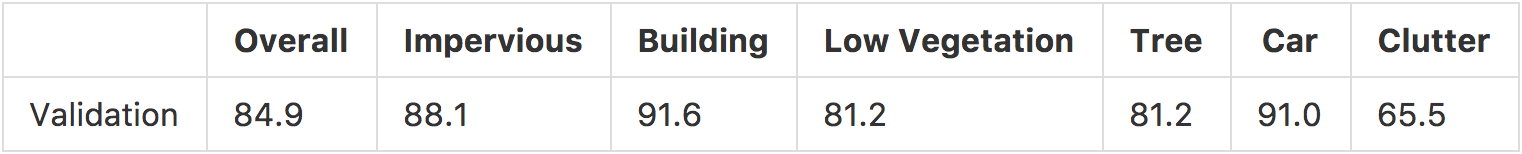
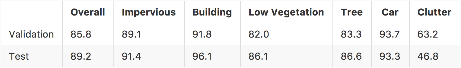
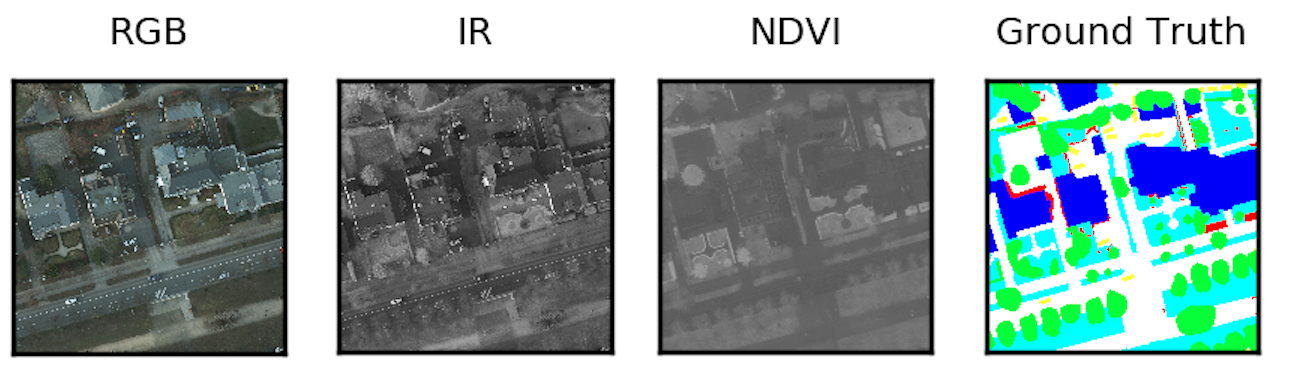
This experiment used a ResNet50-based FCN with connections from the last 32×32, 16×16, and 8×8 layers of the ResNet. We trained the model using a random initialization for 150 epochs with 4096 samples per epoch with a batch size of 8 using the Adam optimizer with a learning rate of 1e-5. The input to the network consisted of red, green, blue, elevation, infrared, and NDVI channels. The NDVI channel is a function of red and infrared channels which tends to highlight vegetation. The training data consisted of 80% of the labeled data, and was randomly augmented using 90 degree rotations and horizontal and vertical flips. The training process took ~8 hrs on an NVIDIA Tesla K80 GPU. The network takes 256×256 windows of data as input. To generate predictions for larger images, we made predictions over a sliding window (with 50% overlapping of windows) and stitched the resulting predictions together. We obtained the following scores on the validation set, which is composed of 20% of the development dataset. The overall score is the accuracy for all labels, and the individual scores are F1 scores.
Here are some predictions from the learned model over a 2000×2000 tile from the validation set. The predictions look generally correct, although the model struggles with the clutter category and finding exact boundaries, especially for the natural categories of low vegetation and trees.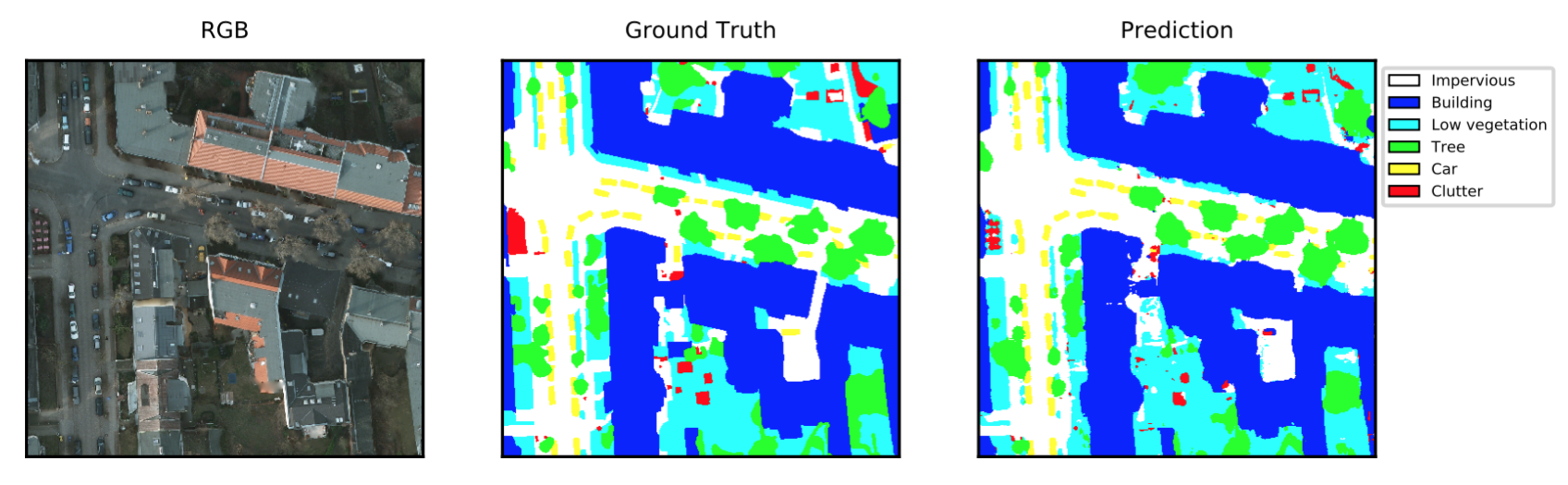
The configuration file for this experiment can be found here and the code for the model here.
Pre-trained ResNet50 with ImageNet on IR-R-G
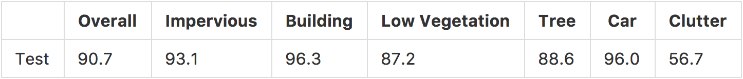
This experiment was the same as the previous, except that it used pre-training, initializing the ResNet with weights learned on ImageNet, and was only trained for 100 epochs. Since the model trained on ImageNet only had three input channels, we could only use three of the available input channels. We chose infrared, red and green. We expected this to perform worse than Experiment 1, because we were ignoring potentially valuable input channels including elevation and NDVI, and because pre-training is typically only useful when there is a small quantity of data, which was not the case. But, surprisingly, there was a 2.4% increase in the accuracy over the previous experiment. The advantage of using pre-training on the Potsdam dataset was first described in this report.
The configuration file for this experiment can be found here.
5-fold Cross-Validation Ensemble
This experiment was the same as the previous except that it trained five models using 5-fold cross-validation, and combined them together as an ensemble. In particular, we trained 5 models, each using a different 20% of the dataset as the validation dataset. The models were then combined by averaging their predictive distributions. Combining models together as an ensemble usually increases accuracy if the ensemble is diverse — that is, if the individual models tend to make different mistakes. In order to increase the diversity of the ensemble, we trained each individual model with a different random initialization (for the non-pre-trained weights in the model), different series of random mini-batches, and different subset of the development dataset. The configuration files for this experiment can be found here.
At the time of writing, the leaderboard for this dataset shows that our best results are in second place behind the best results from the Chinese Academy of Sciences, who achieved an overall accuracy of 91.1. They used a similar approach with the addition of multi-scale inference and the use of ResNet101.
Less Successful Experiments
U-Net
We ran a number of other experiments that didn’t work as well, so will only discuss them briefly. First, we tried the U-Net architecture, which has been successful for biomedical image segmentation and is derived from an autoencoder architecture. It performed better than the FCN trained from scratch using all input channels (Experiment 1), but worse than the FCN using pre-training (Experiment 2), with the following scores.

The configuration file for this experiment can be found here, and the code for the model here.
Fully Convolutional DenseNets
We tried using the Fully Convolutional DenseNet architecture, which is like a U-Net that uses DenseNet blocks. The results were around the same as the U-Net, but took about 8 times longer to train. The configuration file for this experiment can be found here, and the code for the model here.
Late Fusion FCNs
To improve on the results in Experiment 2, we attempted to create a network that combined the benefits of pre-training with the benefits of having access to all the available input channels. We created a new “Dual FCN” architecture that combined a pre-trained ResNet for the infrared, red, and green channels, and a randomly initialized ResNet for the elevation, NDVI, and blue channels. There wasn’t a noticeable improvement though, perhaps because the blue and NDVI channels are redundant, and the elevation channel contains errors. The configuration file for this experiment can be found here, and the code for the model here.
U-Net on Vaihingen
In addition to the Potsdam dataset, ISPRS released a dataset covering the town of Vaihingen, Germany. We ran an experiment using U-Net on the Vaihingen dataset resulting in 87.3% overall accuracy on the test set, but did not put further effort into improving upon this result. The configuration file for this experiment can be found here.
Does NDVI help?
As mentioned previously, we used NDVI as an input channel in some of our experiments because it tends to highlight vegetation, and two of our labels include vegetation.
However, we weren’t sure if it would actually improve accuracy, since NDVI is a function of red and infrared channels, and it’s plausible that the network could discover its own version of NDVI. In order to isolate the influence of the NDVI variable we ran 5 experiments with red, green, and infrared, and 5 experiments with those input channels plus NDVI, keeping everything else the same. The difference in accuracies between the two experiments was not statistically significant, suggesting that there is no advantage to adding NDVI as an input channel on this dataset. One possible explanation to the lack of NDVI’s potential predictive power in this case is that the aerial collection seems to have happened during winter time, as most of the trees are barren of leaves. We plan to test the inclusion of NDVI as a feature in cases where vegetation is more lush to understand if NDVI is a useful feature to include for the classification of vegetation.
Visualization
Scoring metrics like the ones seen above help us understand how our models perform. However, since we are dealing with inherently geospatial data, we naturally want to see it on a map. We can take advantage of tools developed at Azavea like GeoTrellis and GeoPySpark to gain new types of insights into the data and our models. For example, we used GeoTrellis to build a simple viewer that stitches together all the predictions of a set of cross-validated models over the labeled part of the Potsdam dataset and displays them on a map. This allows us to pan and zoom over the entire city, which is more convenient than looking at a series of static images.
The legend for predictions for each of the following visualizations is as follows:

Here we can see the resolution of the imagery, and the supplied labels for the data:
The opacity slider makes it easy to view predictions that are aligned with the input. The animation below shows us comparing the FCN prediction to the RGB imagery as well as the labeled data. Each of the tiles in the prediction layer come from a cross validation set, so that the predictions you see are based on the validation set of that particular cross validation run.
We can also highlight incorrect predictions, view raw label probabilities, and compare the output of different model architectures. In the below visualization, green represents pixels that were labeled correctly by FCN and incorrectly with U-Net, blue pixels are where U-Net got it right and FCN got it wrong, and red is where both of the architectures predicted incorrectly.
This tool has been useful in pointing out issues with input data. For example, we were able to discover that the DSM provided by ISPRS had several triangulation errors and tile boundary errors, which we were able to correct by deriving our own DSM using GeoTrellis and PDAL directly from the LiDAR.
We were also able to derive insights about certain qualities of the models. For example, the U-Net model consistently labeled portions of roads as buildings, especially around intersections. Here we see a visualization of what the model got incorrect, as well as rendering of the model’s output probability that each pixel is a building.
We were also able to see some interesting situations where the model prediction made sense, even though it would be scored wrong. For instance, a large food truck was labeled by the training data completely as the “Car” category, while both the U-Net and FCN architectures saw it as part-car, part-building.
The server and frontend for running the above visualizations can be found in this repository.
Because the input and prediction data was stored on S3 as GeoTrellis layers, we were also able to use GeoPySpark to explore the data more programmatically. Here we are working inside of a GeoNotebook, an open source tool developed by Kitware for visualizing geospatial data in a Jupyter notebook.
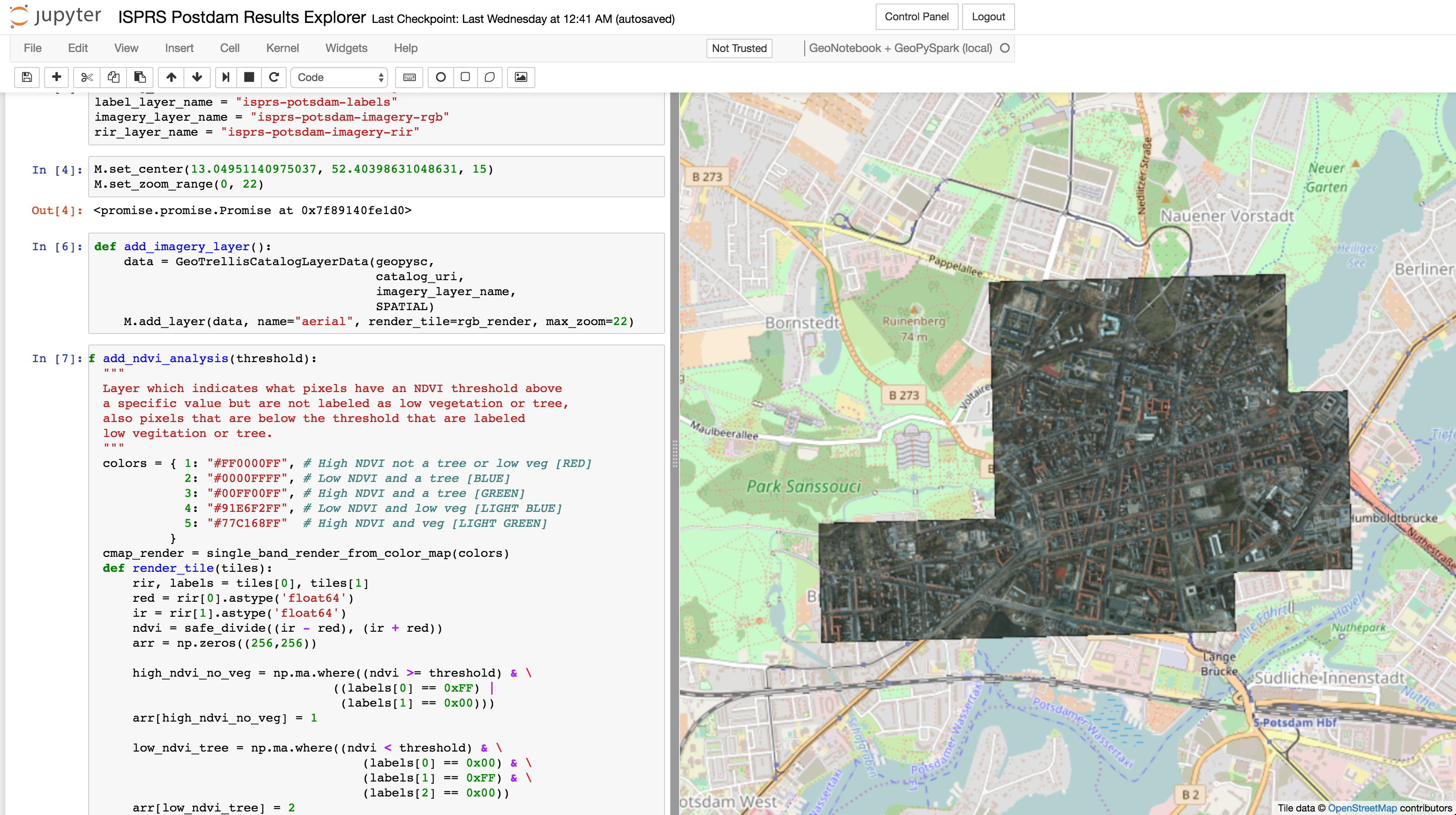
Using the notebook, were able to do interactive analysis on the input data. For example, we viewed areas where NDVI was below a low threshold for pixels that were labeled trees, which indicates that NDVI may not be useful for this dataset. The below animation shows the map updating when changing the NDVI threshold from 0.2 to 0.1. You can see that the portion of the trees hanging over pavement, that have no low vegetation underneath, tend to have low NDVI values.
Future Work
There are a number of potential ways to improve our performance on the Potsdam dataset. We could try using a bigger version of ResNet such as ResNet101, and take the best performing run out of several to help avoid local optima. To make predictions that are less noisy and more spatially coherent, we could try integrating a conditional random field into our model architectures. We could also try re-training our “Dual FCN” architecture on the cleaner GeoTrellis generated DSM.
The Raster Vision project will continue to grow past the ISPRS challenge towards becoming a general platform for performing computer vision tasks on satellite and aerial imagery using deep learning. We are currently working to enable training and prediction for other computer vision tasks, such as image recognition and object detection, as well as take advantage of other techniques such as structured learning and generative adversarial networks (GANs). This will allow us to use Raster Vision to extract structured objects such as road networks, detect changes over time such as deforestation, and generate seamless color corrected mosaics from large sets of imagery taken over time. Another approach to try semi-supervised learning, where a very large unlabeled dataset is used to complement a smaller labeled training set. This was shown to be successful in a recent blog post on sentiment prediction.
Infrastructure improvements to allow massively parallel training of models using AWS Batch are already underway. This will allow us to set up experiments programmatically that vary not only in the input and architecture, as we saw in the experiments above, but that also search the hyperparameter space and let us fine tune the models for peak performance.
If you are wanting to use deep learning to analyze your geospatial imagery, we would love to work with you. Let’s talk.
Update (10/2018): Raster Vision has evolved significantly since this was first published, and the experiment configurations that are referenced are outdated. To run semantic segmentation on the ISPRS Potsdam dataset, we recommend following this example in the raster-vision-examples repository.