
GeoTrellis is a Scala library for working with geospatial data in a distributed environment. While powerful, it has a limited user base due to the geospatial community’s preference for other languages such as Python and R. Bringing GeoTrellis to another language has thus been a requested feature of the community.
Well, after nine months of work, the GeoTrellis team is happy to announce the 0.2.2 release of GeoPySpark!
A binding of GeoTrellis, GeoPySpark allows users to work with a Python front-end backed by Scala.
While not all of the details of GeoPySpark’s development will be discussed (those will be saved for future posts), a brief overview of how it works as well as some demos will be presented in this article.
What Are Language Bindings?
Before going over the workings of GeoPySpark, it would be good to step back and look at what language bindings are. A simple definition would be this: A binding is an API written to allow a library or service to be used in another programming language. Bindings are not ports of their respective project, but rather are just wrappers. Meaning they contain an interface in one language which sends its inputs to the source language for processing.
Implementing GeoPySpark
Much of the functionality of GeoPySpark is handled by another library, PySpark (hence the name, GeoPySpark). PySpark itself is a Python binding of, Spark, a utility available in multiple languages but whose core is in Scala. Because GeoTrellis utilizes Spark, we were able to take advantage of the bindings already in place to create GeoPySpark.
Py4J
Py4J is a tool that Spark (and in turn GeoPySpark) utilizes to allow Scala object and classes and their methods to be accessed in Python. This is done by hooking Python up to the JVM where the Scala code is running. Through this port, references to objects can be passed between the two languages.
The GeoPySpark Backend
Below is the __init__ of RasterLayer, a class in GeoPySpark which is used to store and format raw data in a layer.
 def __init__(self, layer_type, srdd):
     CachableLayer.__init__(self)
     self.pysc = get_spark_context()
     self.layer_type = LayerType(layer_type)
     self.srdd = srdd
That srdd attribute it has is an actual Scala class also called RasterLayer. The Scala class is a reflection of its Python counterpart in terms of the methods it has. Thus, the Python class acts as an interface where the user passes in their parameters which are then sent along to Scala via the srdd. This procedure is described in more detail below:
When a method is executed in Python, the following steps are taken:
- The inputs are checked to make sure they are correct.
- Parameters are then passed to
srdd‘s method call. - Each argument is sent over to Scala where the operation is performed.
- The result of the method is returned to Python.
For a more concrete example, let’s look at RasterLayer‘s reproject method.
def reproject(self, target_crs, resample_method=ResampleMethod.NEAREST_NEIGHBOR):
"""Reproject rasters to ~geopyspark.geotrellis.constants.ResampleMethod, optional):
The resample method to use for the reprojection. If none is specified, then
~geopyspark.geotrellis.layer.RasterLayer
"""
resample_method = ResampleMethod(resample_method)
if isinstance(target_crs, int):
target_crs = str(target_crs)
srdd = self.srdd.reproject(target_crs, resample_method)
return RasterLayer(self.layer_type, srdd)
Above is the Python code for reproject. You can see starting on line #613, the input resample_method is tested to make sure it is a known resampling methods and the target_crs has its type changed if need be. Checks like these need to be done on the Python side due to the nature of the stack trace given if an error was raised in Scala.
Once everything is cleared to go, RasterLayer‘s srdd calls its own reproject method, and the parameters are sent to Scala. Here is what reproject looks like in Scala:
   def reproject(targetCRS: String, resampleMethod: ResampleMethod): ProjectedRasterLayer = {
     val crs = TileLayer.getCRS(targetCRS).get
     new ProjectedRasterLayer(rdd.reproject(crs, resampleMethod))
   }
You can see, the Scala method takes almost the same inputs as its Python counterpart. It returns a new instance of its class, one where the data has been reprojected. This new instance is then brought back to Python where it is used to create a new RasterLayer with it being its srdd.
Below is a picture representation of the reproject‘s execution:
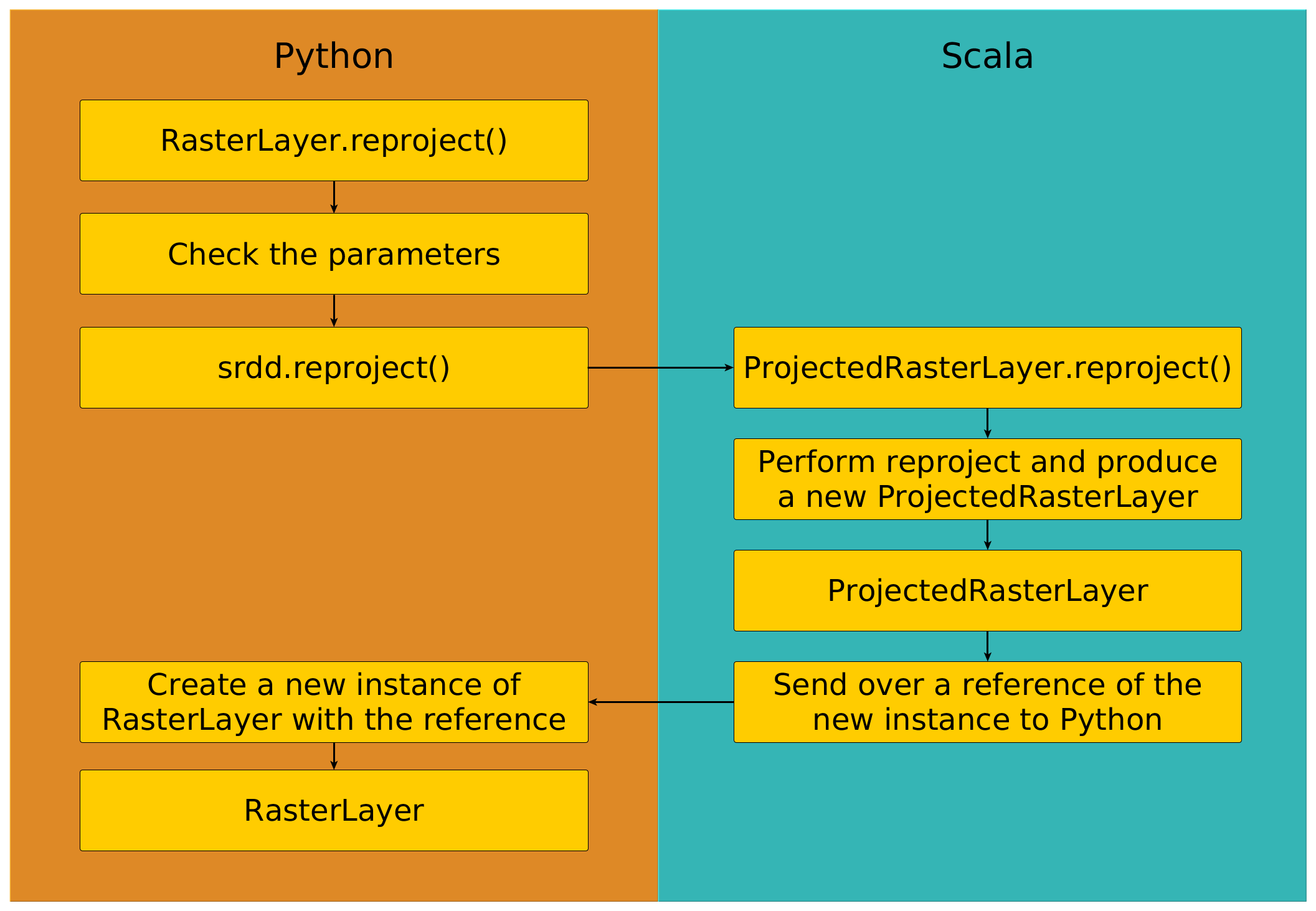
Why would a new instance of RasterLayer be returned and not an RDD? While it’s true that the data is stored and worked within RDDs, sending them back and forth is an expensive and slow process. Instead, the Scala class holds on to the RDD, and will only send it to Python if it is told to do so.
Moving RDDs From One Side to the Other
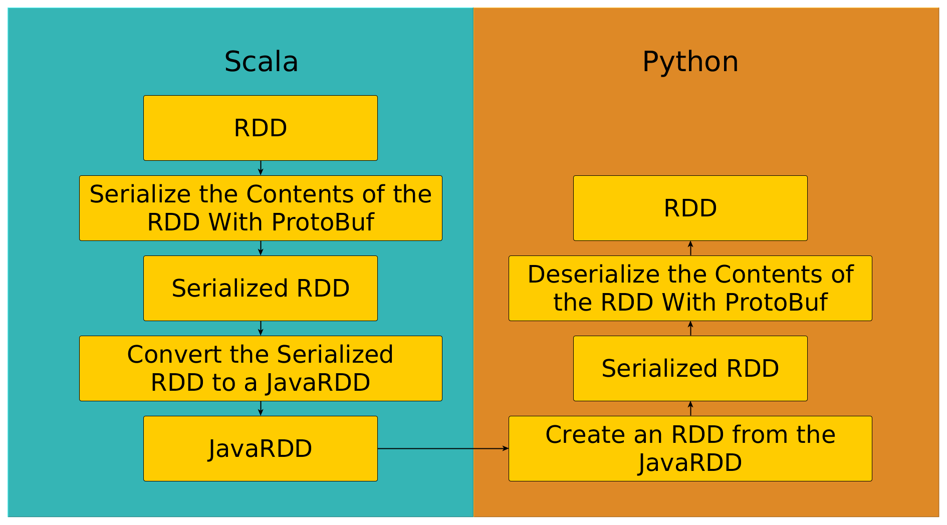
In the previous section, it was mentioned that the process of sending an RDD from Scala to Python is an expensive process. Indeed, the image above illustrates the necessary steps to get our RDD from one side to the other. Notice there is a step that involved turning the RDD into a JavaRDD. This is because in PySpark, an RDD is backed by a JavaRDD which in turn wraps its own Scala RDD.
Before being sent over, the values within the RDD must be serialized. Spark offers different serializers out of the box, however, GeoPySpark uses its own which uses ProtocolBuffers (also known as ProtoBuf). The reason we used ProtoBuf over the built in serializers or other serialization formats is because it’s a fast, language neutral format.
GeoPySpark in a Jupyter Notebook
Jupyter Notebooks is a web application that allows users to create and share documents, called notebooks, with one another. These notebooks can contain live code that can be ran and whose output can viewed in real time.
In order to take advantage of the power of these notebooks, the GeoPySpark team worked with a team at Kitware on their GeoNotebook project. This application is a modified Jupyter notebook that is designed for geospatial processing and analysis. By adding support for GeoPySpark, it is now possible to work with GeoPySpark directly in a notebook.
GeoPySpark in Action
In geospatial analysis, weighted overlays are a technique used to evaluate various factors in order to better understand how geography affects decision making. For instance, if you are looking for a place to live or start a business, you may want to be closer or farther away from certain amenities than others. In this example, a cost distance model will be created where the favorability of three different factors: the location of bars, transit stops, and cafes will be adjusted using the road system as a friction layer in San Francisco. Once calculated, a TMS server will start that will display the weighted, cost distance layer.
Before beginning, make sure that you have the required dependencies to run GeoPySpark. If you are unable to meet these requirements, then there is an alternative discussed more below. In addition to having the environment setup to run GeoPySpark, the required files need to be downloaded as well. To obtain these files, run the following commands in the
terminal:
curl -o /tmp/bars.geojson https://s3.amazonaws.com/geopyspark-demo/MVP_San_Francisco/bars.geojson
curl -o /tmp/cafes.geojson https://s3.amazonaws.com/geopyspark-demo/MVP_San_Francisco/cafes.geojson
curl -o /tmp/transit.geojson https://s3.amazonaws.com/geopyspark-demo/MVP_San_Francisco/transit.geojson
curl -o /tmp/roads.geojson https://s3.amazonaws.com/geopyspark-demo/MVP_San_Francisco/roads.geojson
Once the downloads are complete, the following Python code can be copied and pasted into an editor of your choosing.
from functools import partial
import geopyspark as gps
import fiona
import pyproj

from pyspark import SparkContext
from shapely.geometry import MultiPoint, MultiLineString, shape
from shapely.ops import transform
from geonotebook.wrappers import VectorData, TMSRasterData


def main():

    # Read in all of the downloaded geojsons as Shapely geometries

    with fiona.open("/tmp/bars.geojson") as source:
        bars_crs = source.crs['init']
        bars = MultiPoint([shape(f['geometry']) for f in source])

    with fiona.open("/tmp/cafes.geojson") as source:
        cafes_crs = source.crs['init']
        cafes = MultiPoint([shape(f['geometry']) for f in source])

    with fiona.open("/tmp/transit.geojson") as source:
        transit_crs = source.crs['init']
        transit = MultiPoint([shape(f['geometry']) for f in source])

    with fiona.open("/tmp/roads.geojson") as source:
        roads_crs = source.crs['init']
        roads = [MultiLineString(shape(line['geometry'])) for line in source]


    # Reproject each Shapely geometry to EPSG:3857 so it can be
    # displayed on the map

    def create_partial_reprojection_func(crs):
        return partial(pyproj.transform,
                       pyproj.Proj(init=crs),
                       pyproj.Proj(init='epsg:3857'))

    reprojected_bars = [transform(create_partial_reprojection_func(bars_crs), bar) for bar in bars]
    reprojected_cafes = [transform(create_partial_reprojection_func(cafes_crs), cafe) for cafe in cafes]
    reprojected_transit = [transform(create_partial_reprojection_func(transit_crs), trans) for trans in transit]
    reprojected_roads = [transform(create_partial_reprojection_func(roads_crs), road) for road in roads]

    # Rasterize the road vectors and create the road fricition
    # layer.

    rasterize_options = gps.RasterizerOptions(includePartial=True, sampleType='PixelIsArea')

    road_raster = gps.rasterize(geoms=reprojected_roads,
                                crs="EPSG:3857",
                                zoom=12,
                                fill_value=1,
                                cell_type=gps.CellType.FLOAT32,
                                options=rasterize_options,
                                num_partitions=50)

    road_friction = road_raster.reclassify(value_map={1:1},
                                           data_type=int,
                                           replace_nodata_with=10)

    # Create the cost distance layer for bars based on the
    # road network. Then pyramid the layer.

    bar_layer = gps.cost_distance(friction_layer=road_friction,
                                  geometries=reprojected_bars,
                                  max_distance=1500000.0)

    bar_pyramid = bar_layer.pyramid()

    # Create the cost distance layer for cafes based on the
    # road network. Then pyramid the layer.

    cafe_layer = gps.cost_distance(friction_layer=road_friction,
                                   geometries=reprojected_cafes,
                                   max_distance=1500000.0)

    cafe_pyramid = cafe_layer.pyramid()

    # Create the cost distance layer for the transit stops
    # based on the road network. Then pyramid the layer.

    transit_layer = gps.cost_distance(friction_layer=road_friction,
                                      geometries=reprojected_transit,
                                      max_distance=1500000.0)

    transit_pyramid = transit_layer.pyramid()

    # Calculate the weighted layer based on our preferences.

    weighted_layer = (-1 * bar_pyramid) + (transit_pyramid * 5) + (cafe_pyramid * 1)

    # Calculate the histogram for the weighted layer and
    # then create a ColorRamp from the histogram.

    weighted_histogram = weighted_layer.get_histogram()
    weighted_color_map = gps.ColorMap.build(breaks=weighted_histogram,
                                            colors='viridis')

    # Build the TMS server from the weighted layer with its
    # ColorMap

    tms = gps.TMS.build(source=weighted_layer,
                        display=weighted_color_map)

    print('\n\nStarting the server now\n\n')
    tms.bind(requested_port=5000)


if __name__ == "__main__":

    # Set up our spark context
    conf = gps.geopyspark_conf(appName="San Fran MVP", master="local[*]")
    sc = SparkContext(conf=conf)

    main()
Once you have saved the file, it can be executed with
python [YOUR-FILE-NAME.py]
Where [YOUR-FILE-NAME.py] is whatever you named the file. After a few minutes of running, you will be able to view the results of the analysis by using the TMS server.
To view the results, go to geojson.io and move to the San Francisco
area.
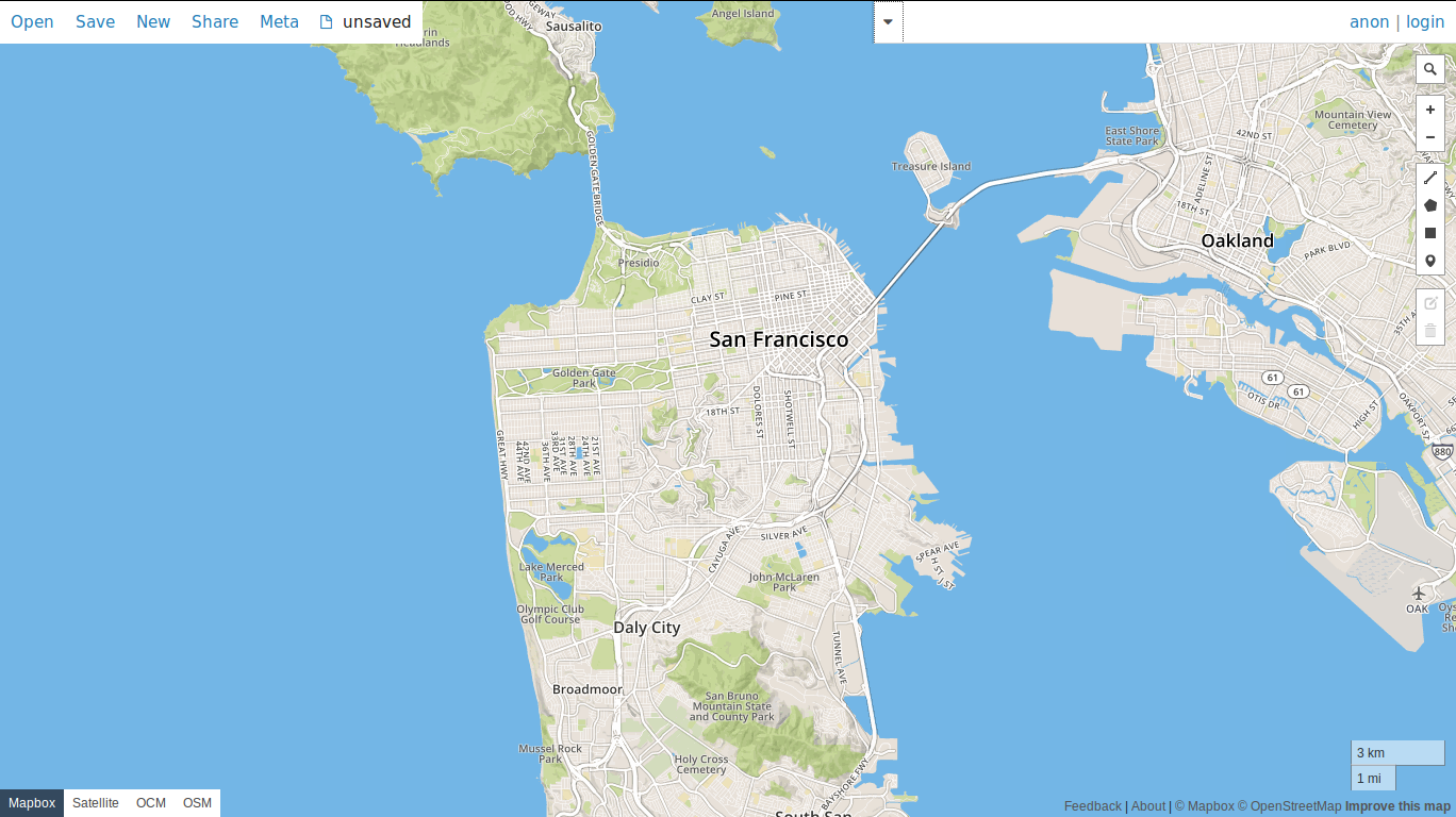
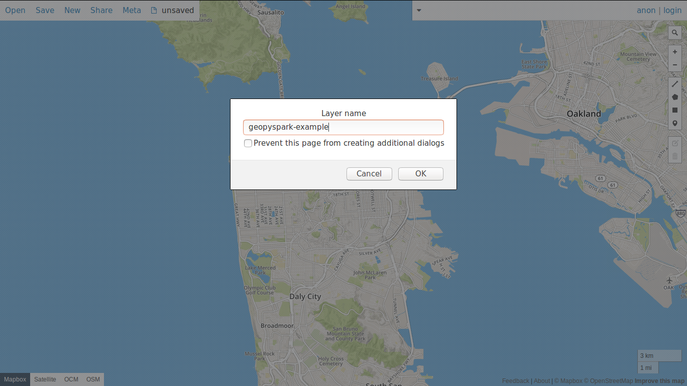
Then select Meta from the toolbar and pick the Add map layer option.
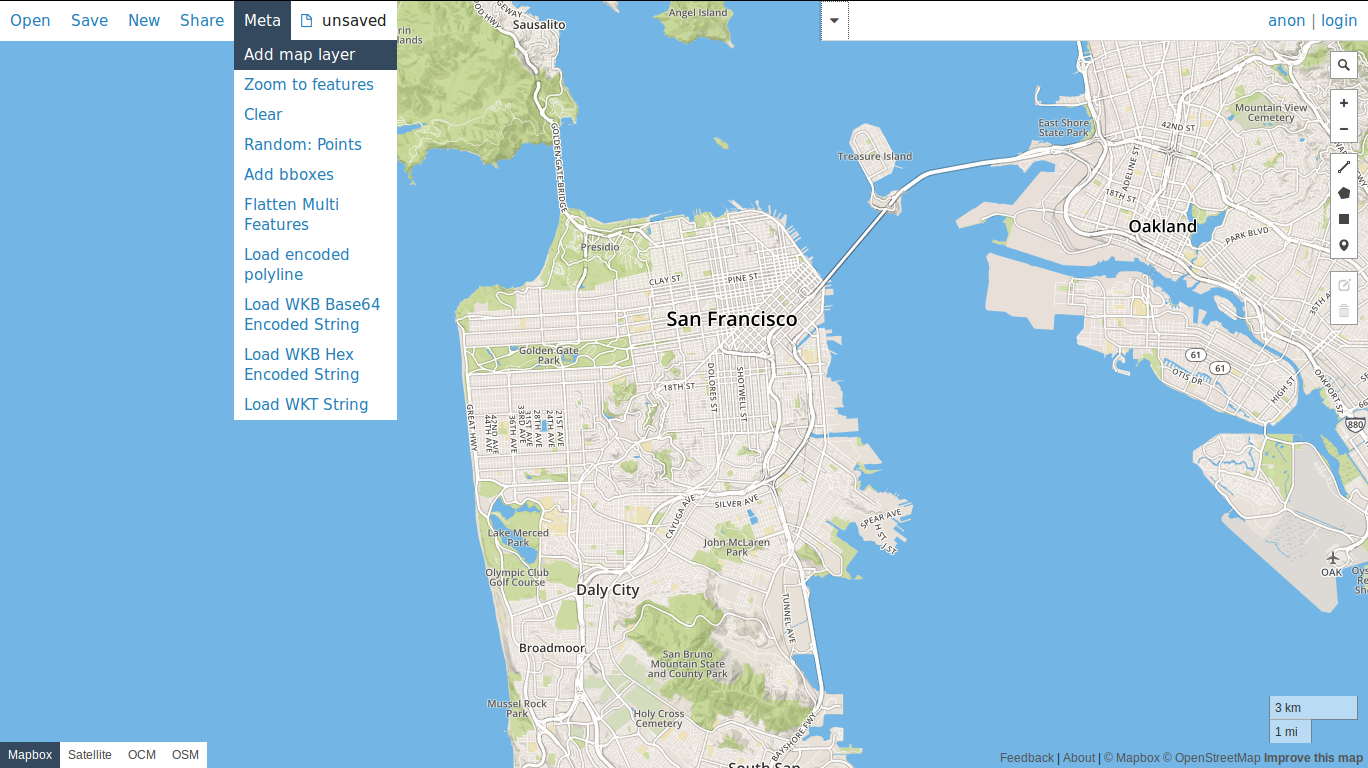
When it asks for the Layer URL, input: http:localhost:5000/tile/{z}/{x}/{y}.png.

Next, for the Layer name, pick anything you’d like. I chose to call the layer,
geopyspark-example.
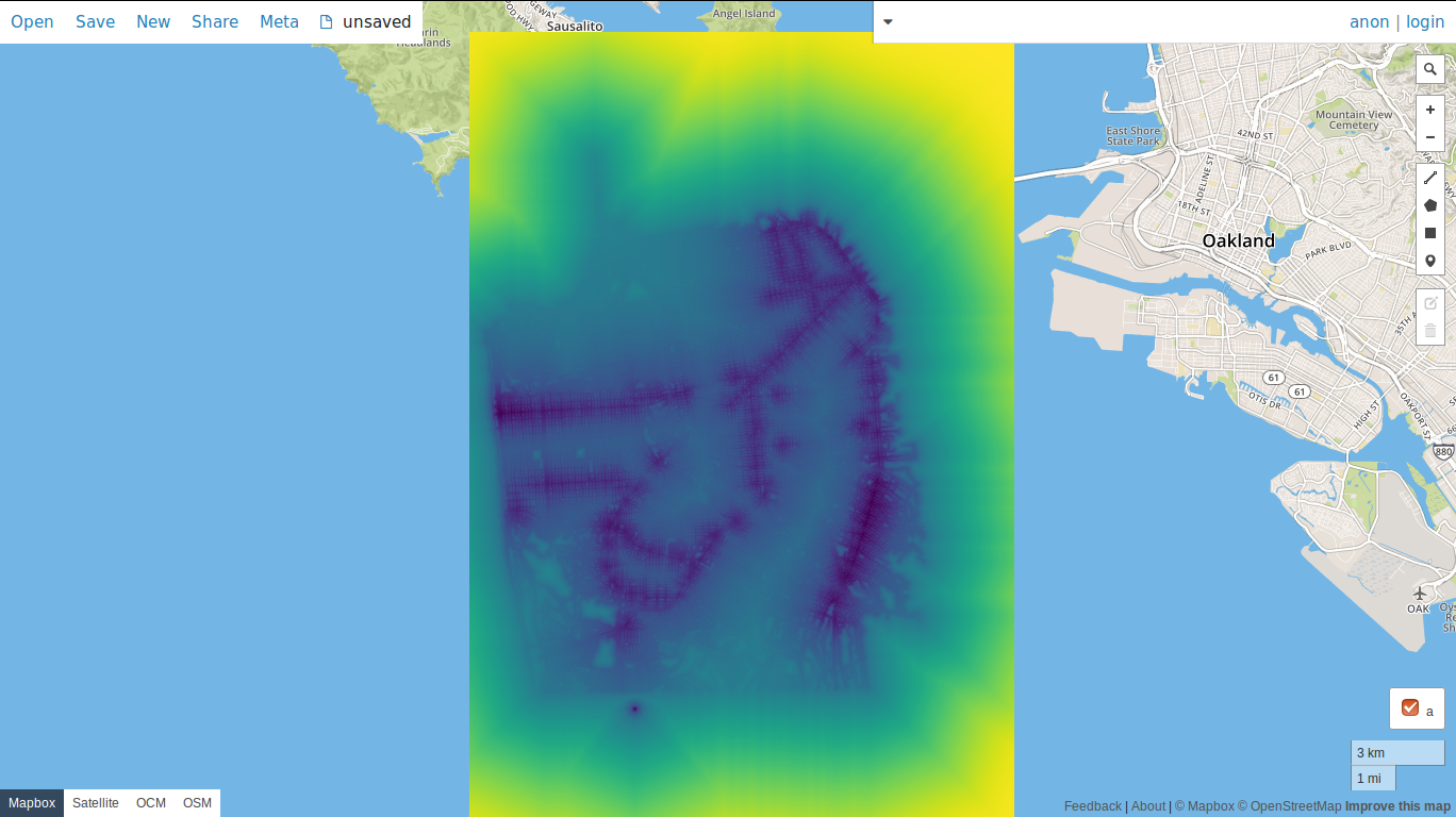
Finally, we should now see the layer on the map.
An Alternative Way of Running GeoPySpark
If you are unable to setup your system to run GeoPySpark, there is another way of using it. The geodocker-jupyter-geopyspark repository contains a docker image that already has GeoPySpark and its dependencies installed and setup. There are also examples of using GeoPySpark (including this previous demo) that can be
worked with in a Jupyter Notebook.
Future Work
While usable in GeoNotebook, there is still work that needs to be done to fully integrate the two, and this is our current focus. Once that is resolved, we plan on continuing GeoPySpark’s functionality by porting more GeoTrellis features over to it.
For more information about how to use GeoPySpark, check out this blog article that goes over how to work with GeoPySpark in a Jupyter Notebook using the above mentioned docker container.