This post is part of a series of articles written by 2016 Summer of Maps Fellows. Azavea’s Summer of Maps Fellowship Program provides impactful pro bono spatial analysis for nonprofits, while fellows benefit from Azavea mentors’ expertise. To see more blog posts about Summer of Maps, click here.

Kriging is a complex and useful tool for GIS analysts. The method presents an array of options and requires a bit of background statistical knowledge. Though there is a wealth of information available online, much of it assumes that the reader already has much of this background information. So, I’m writing the blog post I wish I had found while doing research for my Kriging analysis for my project with the American Red Cross. You can expect:

• A (relatively) jargon-free overview of Kriging
• A workflow for exploring spatial data
• Guidelines for making sure the data meets the necessary assumptions
• Help with defining parameters
• An evaluation of different models using statistical tests

Overview of Spatial Interpolation

Spatial interpolation is a method that uses the known values at given locations to estimate a continuous surface. There are several types of spatial interpolation, including inverse distance weighting (IDW), spline, and Kriging.

Spatial interpolation is useful in a wide variety of contexts, such as estimating rainfall, groundwater pollution, temperature, or the spread of a disease. It helps to ‘fill in the gaps’ between known data points. For example, my project with the American Red Cross, uses Kriging to generate a continuous surface of vulnerability in Liberia based on survey data from specific communities. This surface can then be used to estimate risk even in areas without data.

What is Kriging?

Kriging is a powerful type of spatial interpolation that uses complex mathematical formulas to estimate values at unknown points based on the values at known points. There are several different types of Kriging, including Ordinary, Universal, CoKriging, and Indicator Kriging. This blog post will be focusing on the most common type, Ordinary Kriging.

Ordinary Kriging, as opposed to other types of Kriging, assumes spatial autocorrelation but does not assume any overriding trends or directional drift. Unless you are certain your data exhibits an overarching trend, Ordinary Kriging is generally a good option. I will focus on performing Kriging using ArcMap’s Geostatistical Analyst toolbox. Kriging can also be performed using other software, such as R statistical software, but the Geostatistical Wizard tool in the ArcMap toolbox has an easy-to-use interface.

Prepping the Kriging Model

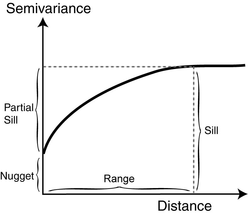
A critical component of generating any Kriging model is creating the semivariogram, which is a plot that shows the variance in measure with distance between all pairs of sampled locations. In the model, points near to each other are expected to be more similar than points that are farther apart. The range is where autocorrelation exists among points based on distance. The nugget is the error or random effect. The sill is the distance at which points are no longer spatially autocorrelated.

While Kriging may be more complex than other types of spatial interpolation, it has greater potential to generate more accurate, validated surfaces. Fitting a Kriging model to data points relies on several assumptions:

1. The data follows a normal bell curve distribution
2. It does not exhibit any overarching global trends
3. It is spatially autocorrelated

 

Normal Distribution

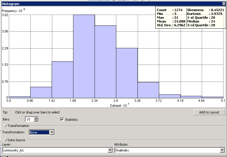
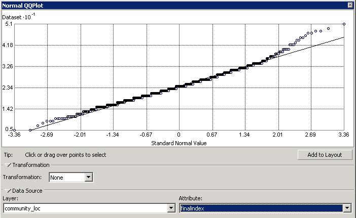
To evaluate if my data points were normally distributed, I created a Histogram and a Normal QQ plot using the Explore Data tool in the Geostatistical Analyst toolbox. The data points followed a bell curve distribution in the Histogram and generally fell along the reference line in the Normal QQ plot. Both of these charts suggest that the data are normally distributed and do not need to be transformed. If my data had not been normally distributed, I could have transformed it using a logarithmic function.

 

Global Trends

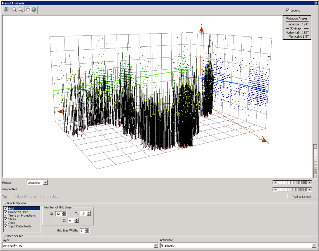
Global trends can interfere with the final interpolation model, so assessing whether the data contains any trends is an important step in the process. To do so, I used the Explore Data tool in the Geostatistical Analyst toolbox to create a Trend Analysis plot that fits a polynomial trend to the data. This interactive 3-D tool allows the user to apply different orders of polynomial trends to the data and visually inspect if the trend seems to fit the data. If the trend fits the data well, the line will be curved upwards or downwards; if the trend does not fit the data well, the line will be horizontal.

None of the polynomial trend lines seemed to fit the data, so I concluded that my data does not exhibit any global trends. If my data had exhibited global trends, I would have needed to remove the trend based on the order of the polynomial. ArcMap’s Geostatistical Wizard provides an option to detrend data based on the necessary polynomial order.

Spatial Autocorrelation

Before creating the Kriging model, I also needed to make sure the data was spatially autocorrelated. To do so, I used ArcMap to perform a Global Moran’s I test on my data to determine whether or not the data exhibits spatial autocorrelation. The resulting z-score of 2.26 and p-value of 0.024 suggest that the data is positively spatially autocorrelated, meaning that the spatial distribution of high values and low values in the dataset are more spatially clustered than would be expected if underlying spatial processes were random.

Creating the Semivariogram

Finally, I needed to specify the lag size and number of lags for the semivariogram model. As a general rule of thumb, the lag size multiplied by the lag number should cover roughly half of the total semivariogram coverage. The Average Nearest Neighbors tool in ArcMap’s Spatial Analyst toolbox can be used to find the average distance between nearest neighbors in the dataset, which is often a good lag size.

Using the Geostatistical Wizard Tool

Now that all of the necessary assumptions have been met, we can finally start creating the Kriging model!

First, open the Geostatistical Wizard tool located in the Geostatistical Analyst toolbar. If you don’t see this toolbar, go to “Customize” and make sure that your “Geostatistical Analyst” extension is turned on.

After opening the tool, select Kriging/CoKriging. Click next and transform your data if it isn’t normally distributed or remove trends if it exhibits any global trends.

Click next to view the semivariogram model that the Geostatistical Wizard automatically generates. This page may look confusing, but let’s just focus on a few key components to help you construct an accurate semivariogram model. There are several different models you can choose from, but the most common models are stable, exponential, and Gaussian. The trend line of the best model will pass most closely through the blue crosses, which represent the averaged values.

Evaluating Kriging Models

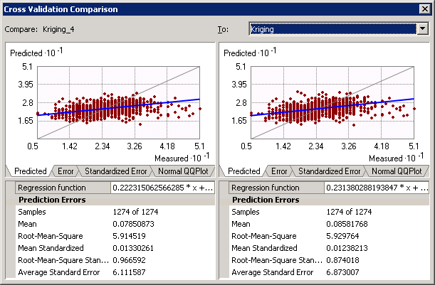
After creating several Kriging models with different semivariogram models, lag sizes, and numbers of lags, I compared these different models using the Compare tool. If you right-click on one of the geostatistical layers, you can select Compare and then change which models are visible in the interface. The Geostatistical Wizard tool cross-validates each Kriging model and calculates several different types of error to help evaluate the model’s accuracy.

Generally, the best model has the following attributes:

• A standardized mean nearest to zero
• The smallest root-mean-square prediction error
• The average standard error nearest to the root-mean-square prediction error
• The standardized root-mean-square prediction error nearest to 1

However, if this seems too complicated, focus on the smallest root-mean-square prediction error because this generally indicates the optimal model. More information about comparing models can be found on ESRI’s website.

Constraining the Geographic Area of the Kriging Model

Though the Geostatistical Analyst toolbar is recommended for actually creating the Kriging model, the Kriging tool in the Spatial Analyst toolbar offers a unique feature that may be helpful. This general Kriging tool allows a user to constrain the interpolation to a specific geographic area, like a city boundary.

To do so, go to the environments settings for the Kriging tool and set a shapefile as a raster mask. Unfortunately the Kriging tool does not give the range of experimental options that the Geostatistical Wizard does. So If you are going to go this route I would recommend using the Geostatistical Wizard tool to experiment with models and determine which semivariogram model, lag size, and number of lags are best, then specify these parameters within the more simple Kriging tool in the Spatial Analyst toolbar.

This way you can get the depth of control from the Geostatistical Wizard while still having the ability to use geographic constraints found with the Kriging tool. More information about Kriging with the Geostatistical Analyst toolbox can be found on ESRI’s website.

Final Interpolated Layers

 

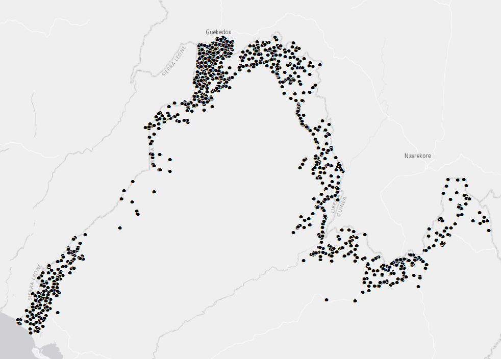
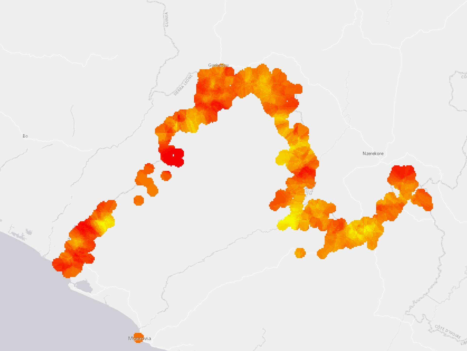
The images above show the original data points and my final interpolated layer of community vulnerability in the border region of Libera. You can see that the surface created is constrained within a specified buffer distance. This was done following the recommendations outline in this post.

The American Red Cross can now use this statistically generated surface to estimate vulnerability and better inform their programming.

Participate in Summer of Maps

Are you a student that’s looking to grow professionally in a GIS analytics career? Do you want to develop spatial analysis skills in a hands-on learning environment?

Keep an eye out for open application dates later this fall and reach out to us with questions about the program!