Automated Building Footprint Extraction (Part 2): Evaluation Metrics

In the first part of this blog series, we discussed the problem of automated building footprint extraction, criteria for what makes a good training dataset, and some examples of open datasets meeting these criteria. In this part, we review some evaluation metrics for building footprint extraction.

Evaluation metrics indicate how well predictions match ground truth labels, and are used to compare the performance of different models. For raster labels, which are typically used in semantic segmentation, evaluation metrics are relatively straightforward and based on the number of pixels that match. With polygonal labels, evaluation metrics are more complex since matching polygons is non-trivial, and polygons vary in complexity and cannot be represented with a fixed-length vector.

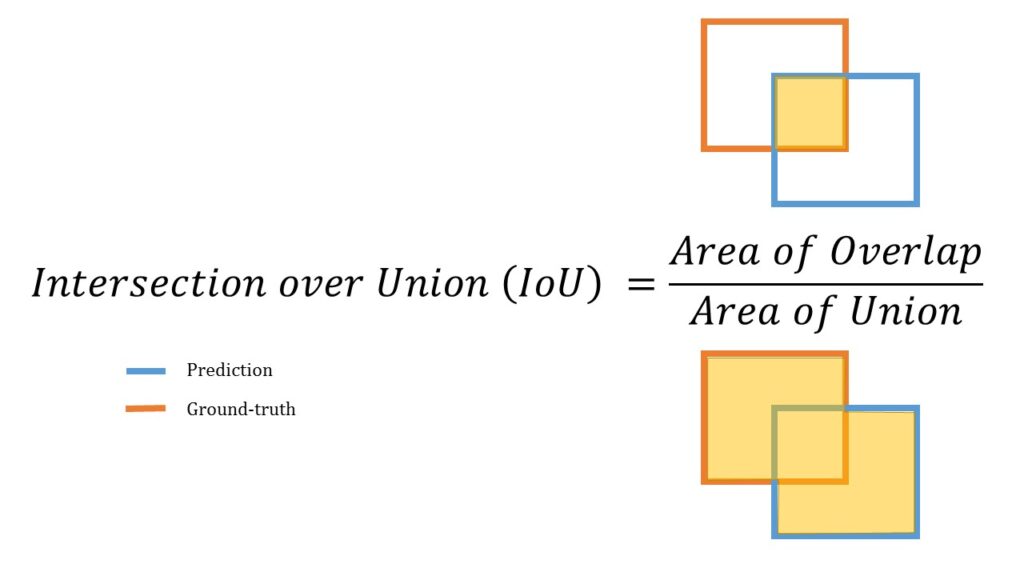
Intersection over Union (IoU)

The simplest metric is intersection over union (IoU), which is the ratio of the area of the intersection over the area of the union of the predicted and ground truth labels. The IoU metric ranges from 0 to 1, and a value of 1 indicates that the predictions perfectly match the ground truth.

COCO Metrics: Average Precision and Recall (AP and AR)

COCO is a popular dataset for object detection and instance segmentation, and is associated with a set of evaluation metrics. These metrics can also be used for building footprint extraction which is a special case of instance segmentation. To compute average precision (AP), the first step is to attempt to match each prediction with a ground truth polygon based on IoU, which must exceed a certain value to be considered a match. If a prediction matches, it is considered a true positive. Otherwise, it is a false positive. Any unmatched ground truth polygons are considered false negatives. Then, precision and recall values can be computed based on the counts of true positives, false positives, and false negatives.

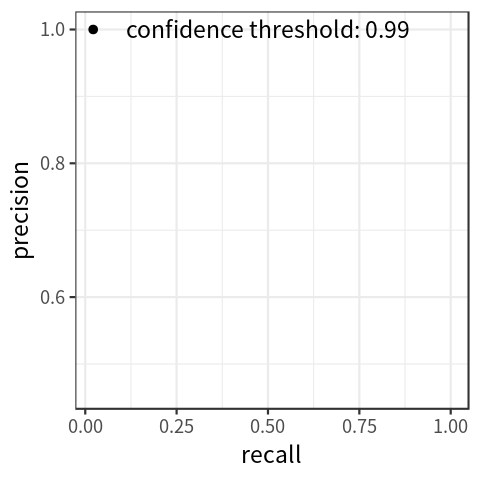
Each prediction is associated with a probability which indicates the model’s confidence in that prediction. By only keeping predictions above a certain probability threshold, recall will decrease, and precision will usually increase. Thus, precision and recall can be traded off by varying this threshold. The performance of a model across all probability thresholds can be visualized using a precision-recall curve, as seen in the figure below. This curve can be summarized in a single number by computing the area under the curve, which is the average precision across all recall values. In practice, a smoothed out version of this curve is used to calculate this value. Different versions of the AP metric can be computed by changing the IoU threshold used for matching, averaging AP over a range of IoU values, or by filtering by object size.

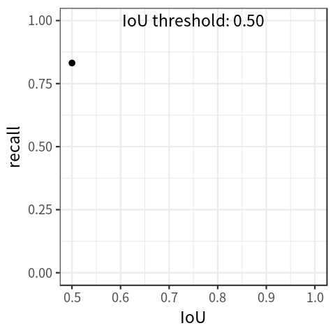
Gif of a line graph demonstrating the tradeoff between precision and recall as the score threshold is varied. As recall increases, precision first drops rapidly, then increases up to ~0.50, and then drops again down to almost 0. — The tradeoff between precision and recall as the score threshold is varied. (Source)

Another metric, average recall (AR), is computed in a similar fashion to AP. This metric is computed by filtering the number of predictions to the top K (eg. 100) based on probability, and measuring the recall across a range of IoU thresholds. This implies a recall-IoU curve, seen in the plot below. Similar to AP, the area under this curve is the average recall (AR) value across IoU values.

Gif of a line graph showing recall decreasing as the IoU threshold increases. — Recall decreases as the IoU threshold increases. (Source)

To learn more about the COCO metrics, see this blog post. The torchmetrics library has an open source implementation of AP and AR.

Max Tangent Angle Error

A downside of the previous metrics is that they fail to adequately penalize predictions that roughly overlap ground truth, but have rounded edges when they should be square. To account for this type of error, the max tangent angle error (MTAE) was introduced. This metric can be computed for a pair of polygons that match based on IoU. To compute it, points are sampled uniformly along the predicted polygon, and each point is matched to the closest point on the ground truth polygon. For each point, the angle of the tangent to the polygon at that point is calculated. Then, the absolute difference (or error) between the angles is calculated for each pair of points. The maximum of these values is the MTAE. For more details, see the appendix of [2].

The max tangent angle error (MTAE) is calculated for two slightly different predictions with the same ground truth. a) On the top row, the prediction is offset from the ground truth, but has square corners that match. On the bottom row, the prediction has a beveled edge instead of a corner on the bottom right. This leads to a greater (ie. worse) MTAE. b) Predicted and ground truth contours from the inset area are juxtaposed. Corresponding sampled points along the contours use the same color. The arrows show the tangents along the contour. c) The error of the angle for each sample point is shown with the maximum value highlighted.

Complexity Aware IoU (cIoU)

Another metric which attempts to correct a deficiency in IoU is Complexity Aware IoU (cIoU) which strikes a balance between segmentation accuracy (measured by IoU) and polygon complexity. By maximizing IoU, models tend to produce excessively complex polygons, whereas buildings typically have a relatively small number of vertices. A straightforward way of measuring the complexity of a polygon is with the count of its vertices, denoted by N_x for polygon x. The cIoU metric scales the IoU value for a pair of predicted and ground truth polygons by the relative difference in the complexity of the polygons. The relative difference between polygons x and y is RD(x, y) = |N_x – N_y| / (N_x + N_y), and the overall metric is IoU * (1 – RD(x, y)). For more information, see the appendix of [3].

The cIoU is calculated for two slightly different predictions with the same ground truth. The cIoU value is lower (ie. worse) for the bottom row where the prediction has a beveled edge.

To learn about model architectures for building footprint extraction, check out the third, and final, part of this blog series. If you missed part one, you can read more about open datasets here.