
Labeling data is hard, time-consuming, and boring. Indeed, much of machine learning research has been, and continues to be, driven by the desire to make do with labeling as little data as possible. While techniques such as self-supervised and semi-supervised learning have received much attention lately, Active learning [1] remains relatively under-explored. Active Learning attempts to reduce the labeling cost by directing the labeling effort towards parts of the dataset that are most useful for improving model performance. Human-in-the-loop active learning (or HITL for short) involves iteratively training a model and getting a human labeller to label new data that best addresses the model’s weaknesses.
As creators of both a geospatial annotation tool, GroundWork, and a geospatial deep learning library, Raster Vision, we found ourselves well-positioned to begin building out this capability. This blog discusses how the HITL workflow works at present, the results it produces, and how it may evolve in the future.
How the label-train-label loop works
Let’s see how the loop works. For concreteness, we will use the example of segmenting cars in a scene from the ISPRS Potsdam Dataset.
Step 0: Label a small initial training set
To start off, we need a small initial training set to train our very first model. This training set need not be very high quality, but, ideally, it should have at least a few instances of the target class(es) so that the model can get some idea of what to look for.
Step 1: Train a model
Next, we use Raster Vision to train a model on the labels we just created.
This training is straightforward for the most part, but there are a few things worth considering:
- Starting model weights: In each round of training, we have a choice of whether to train a new model from scratch or to take the model from the previous round and continue training it with new data. In our experiments (discussed below), we found the latter approach to work better. However, it does have the potential disadvantage that if the model learns something incorrect in earlier rounds, it might not be able to unlearn it in later rounds.
- Data sampling: While using the same model in each round works well, it does introduce the complication that the model will be exposed to some parts of the scene more often than others. For example, a GroundWork-task that was labeled as part of the initial training set will show up in the training data in all subsequent rounds, while one labeled in the last round will show up in just that round. Currently, we do not do anything special to address this, but a potential solution is to assign higher sampling priority to newly labeled tasks.
- Training pool: As we create more labels in each round, our pool of available training data grows. We should take advantage of this to also increase the number of data samples we use for training in each round. Currently, we scale the number of data samples linearly with the number of labeled GroundWork-tasks.
Step 2: Make predictions over the entire scene
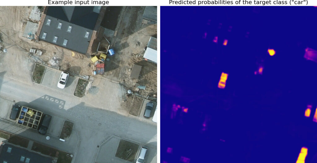
The next step is to identify the model’s weaknesses. To do this, we first use the model to make predictions over the entire scene.
Since this is a semantic segmentation task, the predictions we get are in the form of a probability raster where the value of each pixel represents how likely it is to be part of an instance of the target class (in this case, “car”).
Step 3: Compute labeling priorities
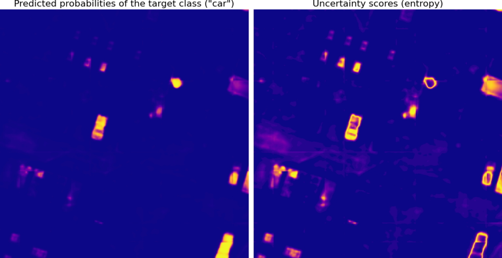
We now want to use the model’s predictions to identify its weaknesses so that we can prioritize labeling regions which will most effectively address those weaknesses. The most common way to do this is to use uncertainty sampling which prioritizes regions where the model is least confident.
To convert probabilities to uncertainty scores we use the entropy function which assigns the highest values to probabilities close to 0.5.
Note that this is not the only way to define “uncertainty”. We can also, for example, train multiple models and define uncertainty to be the areas where they most disagree, but that is obviously much more expensive.
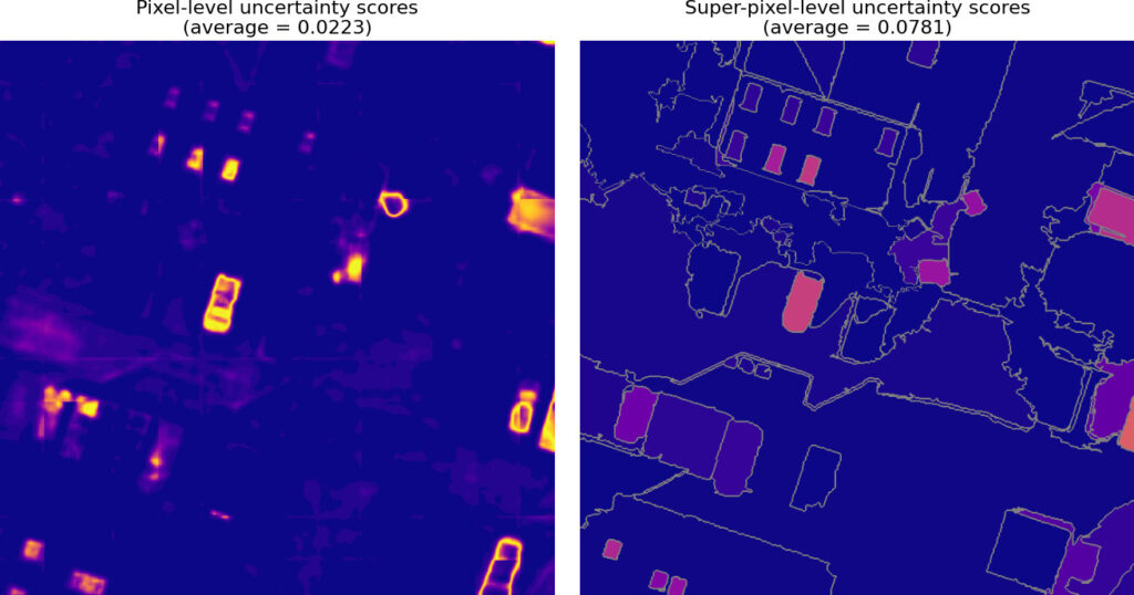
Once we have the uncertainty scores, the final step is to realize that we cannot expect a human to correct labels pixel-by-pixel, so we need to aggregate these pixel-level scores to the task-level.
One simple way to do this is to just average the values of all the pixels in that task, but it has the disadvantage that a large number of small values (the dark blue pixels in the example shown above) can dominate the average, drowning out the signal from the more interesting pixels.
An alternative approach [2] that somewhat avoids this problem is to first aggregate the values to a super-pixel level and then average the super-pixel values.
Regardless of how we do it, we will end up with a prioritized task-grid as shown below.
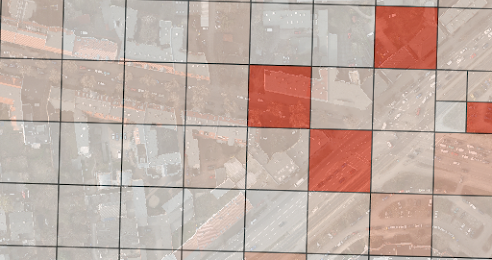
Step 4: Label highest priority areas
With a prioritized task-grid in hand, the next round of labeling is straightforward: we just take some number of the highest priority tasks and label them.
Repeat: Go to Step 1
At this point, we again have a new training set and can repeat the loop starting from Step 1.
Experiments and results
Below we describe some experiments that we performed to shape our intuition about this kind of active learning workflow.
Each experiment involved 5 rounds of labeling and training, with 5 regions of size 512×512 being labeled and added to the training set in each round. Each experiment was run 3 times and used the same model, initial labeled training set, and training and prediction configurations (unless stated otherwise). The reported numbers were computed on a held-out test scene. The same training and test scenes were used in each experiment; both from the ISPRS Potsdam Dataset.
For each experiment, we report here the F1 score (averaged over 3 runs) for the target class (“car”) at the end of each iteration. The error bars represent 95% confidence intervals. In each case, the end of the 5-th round of labeling corresponds to only about 4.5% of the total scene being labeled.
Uncertainty sampling vs. random sampling
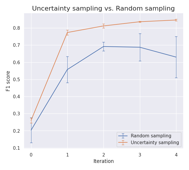
Perhaps the most important question is how uncertainty sampling compares against a baseline approach of randomly selecting which regions to label next.
As it turns out, uncertainty sampling can potentially significantly outperform random sampling depending on the nature of the scene as shown in the plot below. Roughly, the improvement over random sampling depends on how useful any random chip from the scene is for training. If the classes are not too imbalanced and any randomly drawn chip is likely to have a good mix of them (and thus be useful for training), then the gain from uncertainty sampling is small. On the other hand, if, for example, the target class is sparsely distributed within the scene and any randomly drawn chip is likely to be all background, then uncertainty sampling can greatly improve results – this is the case for the example shown below.
Training a new model each round vs. fine-tuning the same model
As discussed above, one important hyperparameter is the choice of the starting weights of the model – whether to start with a fresh model or to use the trained weights from the previous iteration. As shown below, we found the latter to work better.

Super-pixel-based uncertainty aggregation
Above, we discussed two approaches to aggregating the pixel-level uncertainty scores: direct aggregation of all pixel values vs. an aggregation to the super-pixel level followed by an aggregation of the super-pixel values. Below we compare the two approaches and find that super-pixel-based aggregation does not seem to provide any benefit – at least in the example considered here.
Try it out!
An experimental version of the human-in-the-loop functionality is available in GroundWork right now upon request. You can sign up for GroundWork at https://groundwork.azavea.com/ and request human-in-the-loop access by either messaging us in-app or filling out this contact form: https://groundwork.azavea.com/contact/.
What’s next?
On the GroundWork side, there are a few improvements we hope to make:
- Add human-in-the-loop support for the other two computer vision tasks: chip classification and object detection.
- Allow users to customize the training and prediction configuration so that they can tailor it to their specific data.
- Add more visualizations so that users can better examine model predictions and compare model performance across different rounds.
On the research side, we are also interested to see how much more we can get out of a human-in-the-loop workflow by combining it with other reduced-supervision approaches such as self-supervised and semi-supervised learning.
We have shown that an active learning approach can help us get to a high level of model performance with very little data. Not only does it reduce the total number of labels needed, but it also speeds up labeling since tweaking the model’s predictions into the right shape is usually quicker than creating labels from scratch. Moreover, being able to iteratively examine and correct the model’s weaknesses can be incredibly insightful.
We are excited to introduce this capability to the geospatial domain and eager to see how it shapes the future of innovation in the field.
Acknowledgements & References
This capability was developed collaboratively by Aaron Su, Simon Kassel, and the author.
This work was also presented at FOSS4G 2022 and at SatSummit 2022 under the title “Human-in-the-loop Machine Learning with Realtime Model Predictions on Satellite Images”.
[1] Settles, Burr. “Active learning literature survey.” (2009).
[2] Kasarla, Tejaswi, Gattigorla Nagendar, Guruprasad M. Hegde, Vineeth Balasubramanian, and C. V. Jawahar. “Region-based active learning for efficient labeling in semantic segmentation.” In 2019 IEEE Winter Conference on Applications of Computer Vision (WACV), pp. 1109-1117. IEEE, 2019.