Why care about cloud-native access? 

Understanding efficiency gains in a scalable, cloud-native data-processing environment unlocks an array of new possibilities when dealing with large, complex datasets such as the National Water Model. In this article, we take a deep dive into Zarr and Parquet and determine which is more performant on various time scales. 

The National Water Model (NWM) simulates observed and forecast streamflow over the entire Continental United States, including snowmelt, infiltration, and the movement of water through soil. The format in which the NWM outputs are published was not designed for cloud native access, and does not natively support windowed reads. To access just a small area, users have to download a snapshot of the entire country. By making it accessible over the cloud, scientists, researchers, and other hydrology experts will be able to model and predict more accurately.

This cloud accessibility will lead to better flood prediction. NWM streamflow predictions are a valuable resource in modeling water levels. By making it more accessible and easier to integrate into prediction workflows, we aim to help researchers and experts to make better predictions which leads to systemic changes averting loss of life and property damage from devastating natural disasters.

Once the datasets are more easily accessible, researchers will be able to build upon them, and the democratization will unlock new workflows and innovations. We will see it in near real-time dashboards and assisting in urban planning.

Finally, by establishing a path from NetCDF to cloud-native access, we are led to a data extraction, transformation, and loading (ETL) pipeline that applies to numerous scientific datasets. NetCDF is popular in the scientific and climate communities, and with good reason: it allows for accurate representation of multi-dimensional data and works well with High Performance Computing (HPC) environments. An ETL guide for such a conversion will unlock a large number of datasets in a variety of fields.

National Water Model Reanalysis Dataset

According to NOAA’s Big Data Program documentation:

The National Water Model (NWM) is a hydrologic modeling framework that simulates observed and forecast streamflow over the entire continental United States. The NWM simulates the water cycle with mathematical representations of the different processes and how they fit together. A retrospective simulation model is a model run that joins modern modeling technologies and newer, more complete, datasets to obtain a better understanding of past environments. The NOAA NWM Retrospective dataset is one such retrospective simulation model. This retrospective model contains input and output from multi-decade historical simulations. These simulations used observed rainfall as input and ingested other required meteorological input fields from a weather reanalysis dataset.

NOAA currently has three versions of NWM retrospective datasets. A 42-year (February 1979 through December 2020) retrospective simulation using version 2.1 of NWM, a 26-year (January 1993 through December 2018) retrospective simulation using version 2.0 of NWM, and a 25-year (January 1993 through 2017) retrospective simulation using version 1.2 of the National Water Model.

All these datasets are available in NetCDF format with the newer datasets, the 42-year retrospective, and part of the 26-year retrospective also available in the newer Zarr data format. The multi-year NetCDF files are stored in folders for each year. Each year’s folder contains files for each hour of the year for different product types. A small subset of the listing of these files is shown below. The .comp files shown in the listing are NetCDF files stored in the internally compressed NetCDF format. Each of these product files represents the state of the entire country at a particular time instance. Usually, most queries to the NWM are concerned with specific hydrologic unit regions, referenced by Hydrologic Unit Codes or HUCs, that span a specific time range. And so, to get this specific data the user has to download a large amount of data, most of which will eventually be discarded.

noaa-nwm-retrospective-2-1-pds
├-- model_output
    |-- 1979
    |   |-- ...
    |-- 1990
    |   |-- 1990010100.CHRTOUT_DOMAIN1.comp
    |   |-- 1990010100.GWOUT_DOMAIN1.comp
    |   |-- 1990010100.LAKEOUT_DOMAIN1.comp
    |   |-- 1990010100.LDASOUT_DOMAIN1.comp
    |   |-- 1990010100.RTOUT_DOMAIN1.comp
    |   |-- 1990010200.CHRTOUT_DOMAIN1.comp
    |   |-- 1990010200.GWOUT_DOMAIN1.comp
    |   |-- 1990010200.LAKEOUT_DOMAIN1.comp
    |   |-- 1990010200.LDASOUT_DOMAIN1.comp
    |   |-- 1990010200.RTOUT_DOMAIN1.comp
    |   |-- ...
    |   ├-- 1990122300.RTOUT_DOMAIN1.comp
    |-- 1991
    |   |-- 1991010100.CHRTOUT_DOMAIN1.comp
    |   |-- ...
    |   ├-- 1991122300.RTOUT_DOMAIN1.comp
    |-- ...
    ├-- 2020
        |-- 2020010100.CHRTOUT_DOMAIN1.comp
        |-- ...
        ├-- 2020122300.RTOUT_DOMAIN1.comp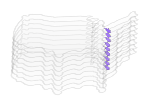

NetCDF format

All the National Water Model (NWM) output created, and disseminated, by NOAA’s Office of Water Prediction (OWP) is in the NetCDF format. The NetCDF format is an excellent format for storing self-describing multi-dimensional datasets reliably and efficiently. However, this file format was created in the eighties when the computing paradigm was very different from what it is today. And, since this file format was designed primarily to meet the needs of climate/meteorological researchers, the NetCDF file format has been in wide use in the geoscience community for a long time.

Despite its tenure, the NetCDF format is not quite suitable for the cloud computing paradigm. The issue is that it is impossible to use the windowed read/write ability which is quite pervasive in cloud computing. This means that using a small subset of data requires downloading the whole .nc file from which you extract only the variables that you need for your analysis.The scientific software stack (eg. the PyData stack which includes NumPy, SciPy, Pandas, scikit-learn, etc.) for the Python language has continued to mature. Additionally, more people are using Python for scientific/numeric computing and using Python along with cloud services (like AWS, GCP, or Azure) to do scientific computing. This is in contrast to the high performance computing (HPC) environments which were the dominant form of large scale computing in the past. The evolution of the PyData stack, and the broader big data ecosystem, has spurred newer data storage specifications/formats that allow for storing and analyzing larger datasets using the cloud computing paradigm. Zarr and Parquet are two such newer data formats.

Zarr format

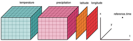
Zarr is a format for the storage of chunked, compressed, N-dimensional arrays.  This format is well-suited for windowed read/writes of multi-dimensional data because it stores arrays using a key/value interface to the underlying data. The key is a string, which is derived from the multi-dimensional indices of the array, and the value is the raw bytes corresponding to the array values of those indices. This dictionary/map-like interface enables flexible windowed reads/writes of the subset(s) of the underlying arrays.  The project’s website details the impressive features that are a part of the Zarr format. The features mentioned in the Zarr storage specification are implemented in different packages in the PyData ecosystem which has made Zarr a popular file format in the geoscience Python community. Various national agencies have also started offering multi-dimensional data in Zarr format includingNOAA’s National Water Model CONUS Retrospective Dataset which is available in Zarr as well as NetCDF.

Parquet format

Parquet is an open-source, column-oriented data storage format. Column-oriented, or columnar, data formats are a storage format where the columns are stored contiguously in memory. This is in contrast to the row-oriented formats (common among most transaction processing databases) where data is stored as a collection of rows where each row is a tuple of heterogeneous data types. Columnar data formats have become hugely popular in the last few years because they are well-suited for analytic use cases. Parquet is one such columnar data format and it has seen immense popularity in the big data ecosystem (especially Apache Spark and Apache Hadoop systems) commonly used in business settings. Parquet is especially suited for tabular workloads where data is organized in 2-dimensional tables of heterogeneous column data types. Since part of the NWM data are tabular in nature, we are interested in comparing Parquet with the Zarr data format.

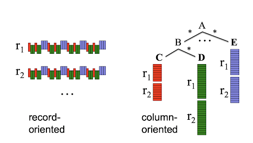
Contiguously stored columns in columnar data formats are better able to use the memory caches and take advantage of modern compression algorithms. They are also specifically designed for the cloud computing paradigm. Both of these characteristics make the Parquet storage format faster and smaller (in physical disk usage size) than record-oriented formats like CSV.

Benchmarking Zarr and Parquet

To gain insight into the performance of different cloud-friendly data formats, we chose a subset small enough to ensure it would not take a prohibitive amount of time to derive any meaningful results, but not so small that it is trivial. So, we decided to run our benchmarks for the HUC2 region that covers the mid-Atlantic, shown below, over a decade of observations.

Data and computing environment setup

Zarr data subset

We extracted a subset of the chrtout.zarr dataset from NOAA’s NWM Retrospective Dataset for our experiments into a smaller dataset. The chrtout.zarr file was subset spatially to the 02 HUC2 (Mid-Atlantic region) boundary, and temporally to the time range of [1990-01-01, 2000-01-01]. This yielded a Zarr dataset with the shape 87672 x 122256. Our goal was to convert this subset into Parquet format using the xarray and dask Python libraries. All of the scripts pertaining to our format conversion and ESIP benchmarking related efforts can be found in the project repository.This original Zarr data subset derived from the above subsetting criteria had a chunk size of 672 24143. To evaluate the impact of different chunking shapes on read/write performance we rechunked this subset using two different chunking schemes: 67230000 and 30000672. The first chunking scheme creates short and wide block arrays (or array chunk shapes in Dask parlance) whereas the second chunking scheme creates long and narrow block arrays. In both chunking schemes the first dimension corresponds to time and the second dimension corresponds to feature_id.

Parquet data subset

We had quite a few difficulties in converting Zarr to Parquet formats. We had a lot of trouble getting xr.DataSet.to_dask_dataframe and xr.DataSet.to_pandas to work reliably on our Dask cluster. Running these functions on our DaskHub cluster with our small test subset resulted in random Jupyter kernel crashes and KilledWorker exceptions. We are unsure of what we are doing wrong and have sought guidance from the community. We have reported the issues we faced to the xarray project and the dask community forum.

Workaround

Since our primary goal was to run benchmarks comparing the Zarr and Parquet formats, we needed to figure out a way to export the Parquet files first. To work around issues with the JupyterHub instance crashing, we extracted data by month and saved the Parquet files for the respective month. Once we had Parquet files for all the 120 months we consolidated them into a single large Parquet dataset using dask.dataframe.concat. While this workaround enabled us to generate the above-mentioned benchmarks, which we reported at the ESIP 2022 conference, we learned that it might be beneficial to store the dataset in wide format. A wide format is where we store each feature_id as a separate column as shown in the tables below. This enables us to select only the features that we need by specifying the list of feature_ids. We first tried converting from long format to wide format using the dask.dataframe.pivot_table on our Kubernetes cluster, but continued to face a variety of errors with Dask and Jupyter. After struggling with distributed Dask cluster-related issues, we decided to generate the wide Parquet dataset on a larger EC2 instance (r5a.4xlarge which has 128GiB of memory). Using dask.distributed.Client, which you can use even on a single multicore computer to use all the cores in parallel, enabled us to create the wide Parquet dataset that we needed. We used the xarray.Dataset.to_pandas instead of pivoting the long format dataset that we had already created. Even with a larger EC2 instance we still had to generate the Parquet files in small subsets (“by year” in contrast to “by couple of weeks” on the Dask cluster), but it was manageable and we could finally create a wide Parquet dataset (where each column corresponds to a unique feature_id). So, finally we had a Parquet dataset with 8762 rows and 122256 columns!

feature_id	time	streamflow
1748535	1990-01-01T01:00:00	0.57
1748535	1990-01-01T02:00:00	0.57
1748535	1990-01-01T03:00:00	0.57
1748535	1990-01-01T04:00:00	0.57
…	…	…
1748537	1990-01-01T01:00:00	1.44
1748537	1990-01-01T02:00:00	1.09
1748537	1990-01-01T03:00:00	0.83
1748537	1990-01-01T04:00:00	0.54
…	…	…
932080037	1990-01-01T01:00:00	1.01
932080037	1990-01-01T02:00:00	0.99
932080037	1990-01-01T03:00:00	0.97
932080037	1990-01-01T04:00:00	0.93

time	streamflow_1748535	streamflow_1748537	streamflow_932080037	…
1990-01-01T01:00:00	0.57	1.44	1.01	…
1990-01-01T02:00:00	0.57	1.09	0.99	…
1990-01-01T03:00:00	0.57	0.83	0.97	…
1990-01-01T04:00:00	0.57	0.54	0.93	…

Computing environment

We used a distributed Dask cluster hosted on Amazon Elastic Kubernetes Service (EKS) to run these benchmarks. The Dask cluster was provisioned by using a custom DaskHub Helm chart.

Benchmarking

To compare the performance of Zarr and Parquet formats we computed the following aggregate variables: mean streamflow per day, mean streamflow per week, and mean streamflow per feature per day. The Python code snippets for generating these aggregates using the xarray package are:

1. Mean streamflow per day:

ds.streamflow.groupby('time.dayofyear').mean()

2. Mean streamflow per week:

ds.streamflow.groupby('time.weekofyear').mean()

3. Mean streamflow per feature per day:

ds.streamflow.mean(dim='feature_id').groupby('time.dayofyear').mean()

Each of these variables was calculated for the time ranges of 1 month (1990-01-01–1990-02-01), 1 year (1990-01-01–1991-01-01), and 10 years (1990-01-01–2000-01-01). These time ranges correspond to 31 days, 365 days, and 3652 days respectively.

1. Mean streamflow per day:

df.groupby(df.index.dayofyear).streamflow.mean().values.compute()

2. Mean streamflow per week:

df.groupby(df.index.weekofyear).streamflow.mean().values.compute()

3. Mean streamflow per feature per day

df.groupby(['feature_id',df.index.dayofyear]).streamflow.mean().values.compute()

Since Parquet is a two-dimensional tabular data format, the above queries, which are for n-dimensional array data, have to be modified to be usable. Below are the above queries modified to be used with the tabular data:

The complete code listing for the benchmarks presented here can be found in this Jupyter notebook.

Benchmarking results

Below are the plots of the benchmarking runs for the various file formats.

Zarr

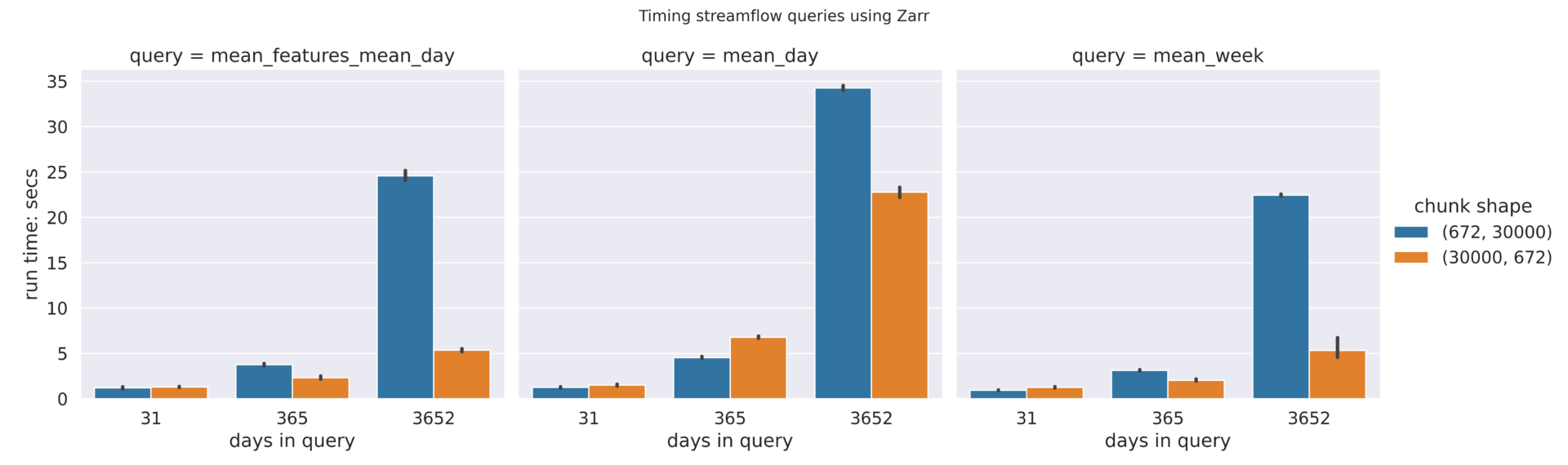
The plot of benchmarking numbers for differently chunked Zarr files shows that a chunking scheme that generates long and narrow (30000672) performs better, at least in the queries that we have used, than a chunking scheme that generates short and wide block arrays (67230000). This result is expected, since our queries involve long time ranges and few feature ids, which requires fetching fewer chunks with the long and narrow chunk shape.

Parquet (long)

A plot of the benchmarking numbers for the long Parquet is below. As described in the table above a long parquet has feature_id and time stored as columns. This long data format is generated by the xarray dataset’s to_dask_dataframe() function.

Parquet (wide)

A plot of the benchmarking numbers for the wide Parquet is below. In contrast to the long format, in the wide format each feature_id is stored as a distinct column. This wide data format is generated by the xarray dataset’s to_pandas() function.

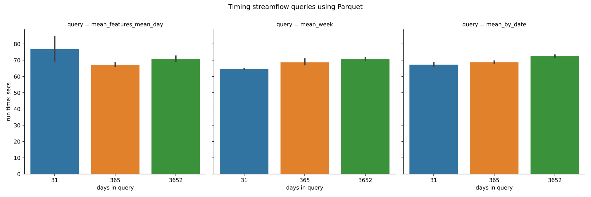
We expected that converting the Parquet file from long to wide format would improve performance. Although the wide format performs slightly better than the long format for Parquet, it is not noticeably different.

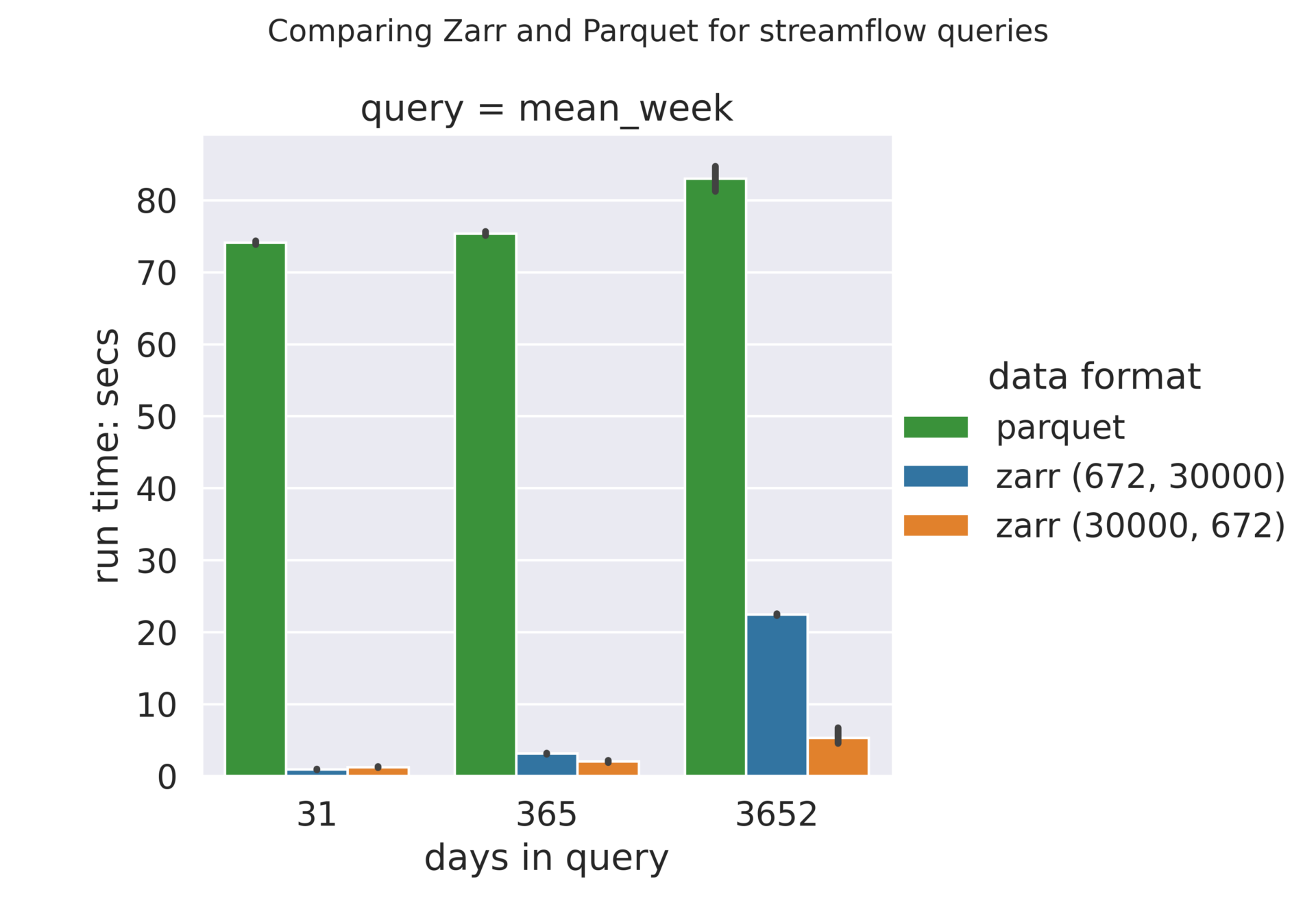
Zarr vs Parquet benchmarks

Displaying the Zarr and Parquet (long) benchmarks side-by-side demonstrates the performance difference between the two formats. Regardless of the re-chunking scheme used, Zarr performed better than Parquet format.

Observations & conclusions

Here are some of the observations we have made:

• For tabular data, Zarr can perform better than Parquet when filtering along multiple dimensions (feature_id and time)
• Chunking Zarr using different schemes impacts read/write performance. In time series queries, a chunking scheme with larger value for time dimension means that there are fewer chunks that need to be read than a chunking scheme which necessitates reading more chunks. These performance differences get more pronounced for larger time range queries.
• In our experiments, Parquet formats, both wide and long, are almost 2x slower than Zarr format! We were expecting Parquet to be faster, or at least on par, with the Zarr format. This is the most surprising finding from our benchmarks! It appears to us that it is quite possible that we are not formatting the Parquet data optimally.
• One curious observation for Parquet format, regardless of its shape, is that the time range queries do not seem to have any effect on performance. That is, the query for the ten years time range takes nearly the same time as the query for one month.

Future & related work

In the future we plan to further our research and understanding through:

• Fixing issues with writing and reading Parquet using Dask
• Running larger experiments
• Benchmarking with other queries
• Saving the entire NWM-R dataset using different formats
• Developing a data access library that automatically selects the best format for a query.

Below are some links to related work which has informed, and inspired us in undertaking our work:

• Cloud-optimized USGS Time Series Data – A blog post demonstrating Parquet outperforming Zarr on a small dataset.
• Why is Parquet/Pandas faster than Zarray/Xarray here? – A Pangeo forum post demonstrating that Parquet is faster than Zarr for streamflow data.
• Pangeo Forge – An open source framework for ETL of scientific data. This framework is primarily focused on the multidimensional array data model rather than the tabular/columnar data model.

We are thrilled to be working with such a curious and brilliant community.

All our work for this is open source, and can be found here: https://github.com/azavea/noaa-hydro-data. We believe in open data, open source, and open science, and welcome all collaborators to offer suggestions and insights.

This work was done with guidance and support from the NOAA community, for which we are grateful. In particular, we’d like to thank Sudhir Shrestha (NOAA), Jason Regina (NOAA), Austin Raney (CUAHSI), and Fernando Aristizabal (Lynker) for their significant counsel and advice.