This Month We Learned (TMWL) is a recurring blog series highlighting what we’ve learned in the last month. It gives us an opportunity to share short stories about what we’ve learned and to highlight the ways we’ve grown and learned both in our jobs and outside of them. This month we learned about effective pair programming, baking and painting tiles with gdal2tiles, adding ways to OpenStreetMap with GPS traces, and how to make nubes.

• 

• 

• 

• 

Effective Pair Programming

Jenny Fung

After some great pair programming sessions this month, I have been reflecting on the mechanics of successful pairing. There is a lot more than meets the eye! You can read a lot about pair programming, but I think successful pairing is a mentality.

In this mentality, people, not the computer problem, are the priority. To explain, when all participants share the same information about and understanding of the problem at hand, everyone can contribute better ideas, questions, and solutions, no matter the difference in their level of expertise in that area of a codebase or in title. It takes time and effort to constantly and actively keep all participants on the same page, but it pays off in many dimensions. Internalize that pairing is an open learning opportunity for everyone. Expect to admit your ignorance in real time. Frankly, I find this socially terrifying to do. I have to remind myself that the alternative, stewing in fear, feels even worse and is less productive before I’m able to take the leap.

So that’s the big picture. What do the mechanics look like in practice? Here are some examples.

Screen sharing is a must

Selected tools should be comfortable for all participants. Ideally, drive control will be shared, all the time or in alternation as possible. For local development, we’ve had good experiences remotely pairing using video chat for face and browser sharing alongside LiveShare on VSCode for collaborative coding. When cruising a remote computer, ssh & tmux allow sharing terminal sessions. Shared terminals are particularly helpful for users of command-line text editors.

Keep talking

Unplanned silence is unlikely if you’re doing it right. Explain everything you are thinking or intending. What questions are running through your head? What is the next piece of information you all need? Do you feel stuck, and why? Share them aloud. If everyone is silent, more than likely your minds aren’t blank, but rather you aren’t sharing.

Freely ask what your pair partners are thinking if there is ambiguity or unplanned silence.

Summarize and resummarize

A lot can happen during a pairing session and it is easy to fall out of sync or forget details. Occasionally summarizing along the way is a good way to stay on track and learn more deeply.

At the end of pairing, make sure you leave on the same page and reflect on what worked/didn’t (a meta retrospective). Capture high-level takeaways in writing immediately afterward. 

Here is an exemplary summary Rocky, an Operations Engineer at Azavea, left in an in-progress pull request after we paired to debug failing signed URL uploads to s3 from a Django/React app:

Pairing summary:
- Worked out issues in the ECS task definition.
- Setup proper CORs rules for the bucket.
- Hit a snag with a 403 Forbidden response with the uploads.
- Relaxed the IAM policy and CORs rules, with no success.
- Followed the entire request / response lifecycle to look for anomalies.
- Setup a dev environment on the staging Bastion w/ an instance profile to replicate the task execution environment.
- In a Django shell, followed https://boto3.amazonaws.com/v1/documentation/api/latest/guide/s3-presigned-urls.html, and then used the resulting payload to successfully upload a file with Paw.
- Put the failed request from Chrome next to the successful request in Paw to see what was different.
- Aligned the request we were making in frontend code to look like the request from Paw, and success 🎉
- Identified that the discrepancies in the request bodies aligned with a discrepancy between our frontend and the legacy code
Our next steps are:
- Jenny will clean things up, including working out the best way to handle the bucket ACL.
- Rocky will take the baton and persist changes to the bucket ACL in Terraform.
- Rocky will tighten up the IAM policy and CORs rules.
- Rocky will take one, final, holistic pass at the entire changeset.

Generating Pyramided Tiles from a GeoTiff with GDAL

Terence Tuhinanshu

In the past, we’ve seen how we can generate pyramided tiles from a GeoTiff with GeoTrellis. This month I learned how to do that with GDAL, using gdal2tiles.py from the May 2020 release of GDAL 3.1.

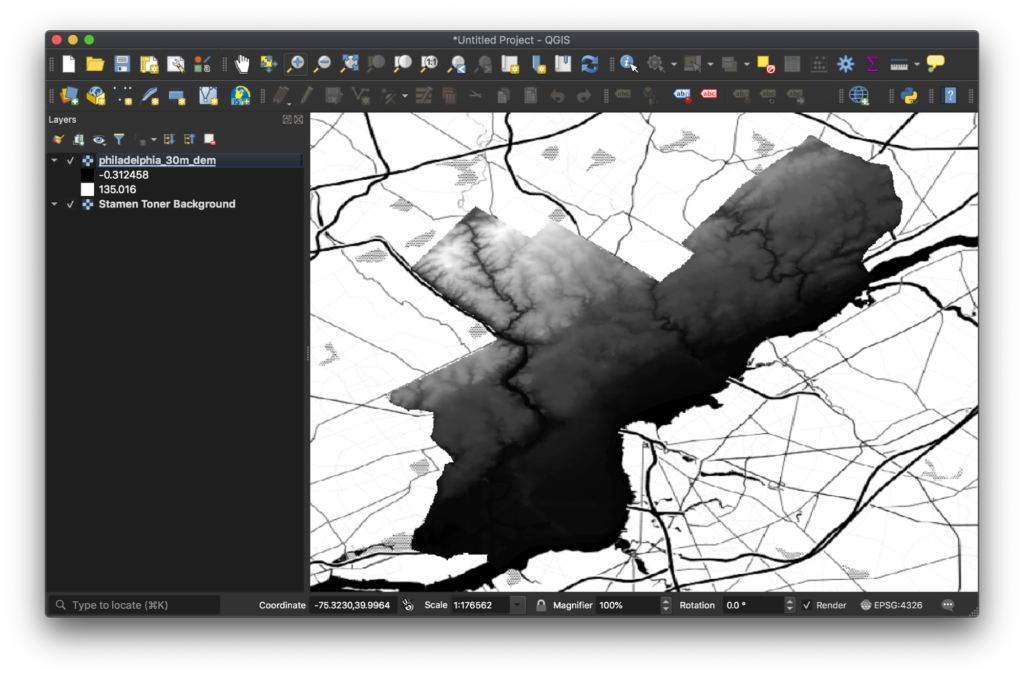
Let’s start with an example GeoTIFF: an elevation dataset from PASDA for Philadelphia county. Downloading and unzipping and loading the file in QGIS, we can visualize it:

Getting the latest GDAL installed on your computer can be challenging. The most straightforward way to do it is to use their Docker image. For our purposes, the most minimal package that will work is the alpine-normal-3.1.0 tag which is about 66 MB.

Create a directory for this project, and cd into it:

$ mkdir ~/gdal-tile-exercise
$ cd ~/gdal-tile-exercise

Make a data directory, and copy over the GeoTIFF into it:

$ mkdir data
$ cp $GEOTIFF_LOCATION data/

Now we can load this directory into the GDAL Docker image and play with it:

$ docker run --rm -it -v $PWD/data:/data osgeo/gdal:alpine-normal-3.1.0 /bin/sh
/ $ cd /data/
/data $ gdalinfo philadelphia_30m_dem.tif
Driver: GTiff/GeoTIFF
Files: philadelphia_30m_dem.tif
Size is 989, 1133
Coordinate System is:
PROJCRS["NAD_1983_Albers",
…

So we have GDAL working, and the file loaded and ready to go. As can be seen in the output above, the current file is in the NAD-1983-Albers projection. We’ll have to reproject it to WebMercator, or EPSG:3857, to be rendered on the web. Then we’ll color the GeoTIFF with a different ramp. Finally, we’ll make the pyramided tiles.

Let’s use gdalwarp to reproject the file:

/data $ gdalwarp -co TILED=YES -co COMPRESS=DEFLATE -t_srs EPSG:3857 philadelphia_30m_dem.tif philadelphia_30m_dem_3857.tif
Creating output file that is 1023P x 1167L.
Processing philadelphia_30m_dem.tif [1/1] : 0Using internal nodata values (e.g. -3.40282e+38) for image philadelphia_30m_dem.tif.
Copying nodata values from source philadelphia_30m_dem.tif to destination philadelphia_30m_dem_3857.tif.
...10...20...30...40...50...60...70...80...90...100 - done.

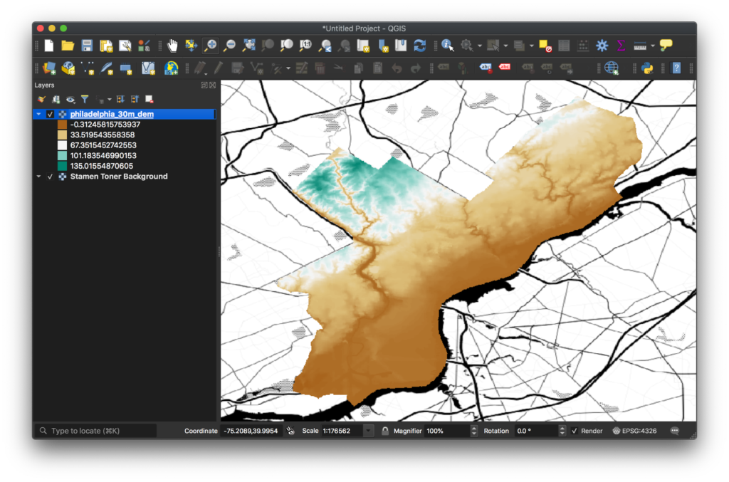
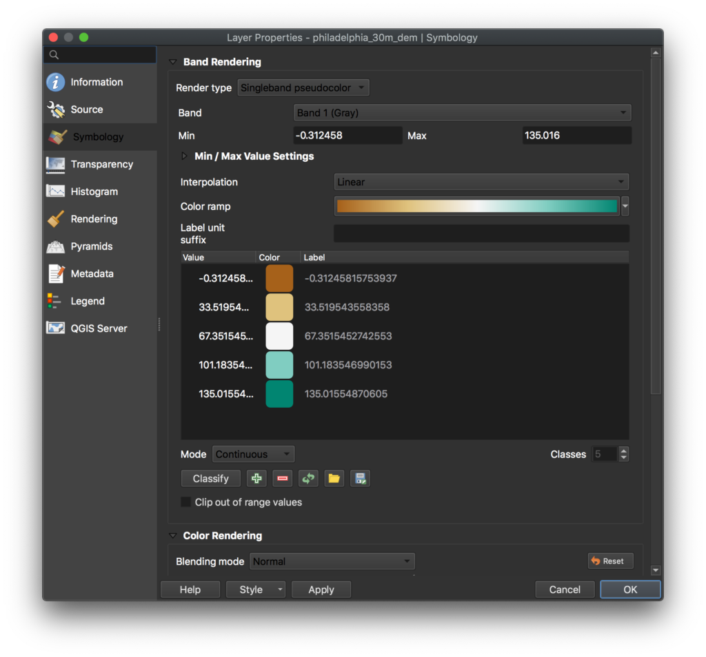
Next, let’s pick what colors it should have. We can use QGIS to see what looks best. In QGIS, right-click the layer and select Properties. Then, under Symbology, switch the Render Type to Singleband Pseudocolor, and pick a color ramp. I picked BrBG, which goes from Brown to Blue-Green and looks nice:

From the Properties dialog you can export the color ramp to a file. Export it to ~/gdal-tile-exercise/data/qgis-colors.txt:

It should be accessible within the GDAL Docker container:

/data $ cat qgis-colors.txt
$ QGIS Generated Color Map Export File
INTERPOLATION:INTERPOLATED
-0.312458,166,97,26,255,-0.31245815753937
33.5195,223,194,125,255,33.519543558358
67.3515,245,245,245,255,67.3515452742553
101.184,128,205,193,255,101.183546990153
135.016,1,133,113,255,135.01554870605

To color the GeoTIFF, we’ll use gdaldem’s color-relief command. This command takes a color configuration file which has a slightly different format from what we exported. To get this into the GDAL format, we need to drop the first two lines, drop the last column of values, and replace commas with spaces:

/data $ sed '1d;2d' qgis-colors.txt | cut -d, -f1-5 | sed 's/\,/ /g' > colors.txt
/data $ echo 'nv 0 0 0 0' >> colors.txt
/data $ cat colors.txt
-0.312458 166 97 26 255
33.5195 223 194 125 255
67.3515 245 245 245 255
101.184 128 205 193 255
135.016 1 133 113 255
nv 0 0 0 0

Here, the first column is the stop, and the next four are RGBA values. If the A value is not specified, it defaults to 255, or full opacity. The final line is added for NODATA values, which should render as transparent in the output, and have their opacity set to 0. Using this file, we can now generate a colored file:

/data $ gdaldem color-relief -alpha -of PNG philadelphia_30m_dem_3857.tif colors.txt philadelphia_30m_dem_3857_colored.tif
0...10...20...30...40...50...60...70...80...90...100 - done.

Finally, let’s make a tiles directory and generate the tiles:

/data $ mkdir tiles
/data $ gdal2tiles.py --zoom=0-13 --resampling=near --processes=4 --xyz philadelphia_30m_dem_3857_colored.tif tiles/
Generating Base Tiles:
0...10...20...30...40...50...60...70...80...90...100
Generating Overview Tiles:
0...10...20...30...40...50...60...70...80...90...100

The --xyz argument is key, which makes Slippy Map Tiles instead of TMS tiles. This was added by Lorenzo Alberton and Even Rouault in OSGeo/gdal#2359, released in GDAL 3.1 in May 2020.

Edit the generated ~/gdal-tile-exercise/data/tiles/leaflet.html to set tms: false in the Overlay layer:

// Overlay layers (TMS)
var lyr = L.tileLayer('./{z}/{x}/{y}.png', {tms: false, opacity: 0.7, attribution: "", minZoom: 0, maxZoom: 13});

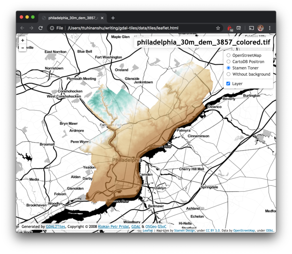
Finally, we can see open this file in the browser and see our tiles 🎉:

OSM Changesets with GPS Tracks

Andrew Fink-Miller

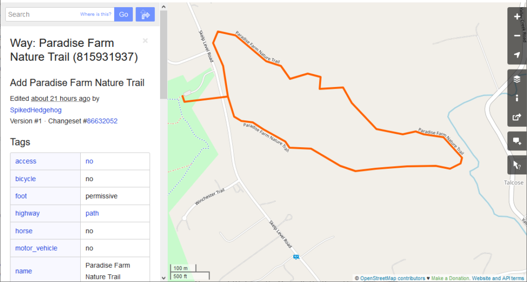
I’ve contributed to OpenStreetMap (OSM) in the past but mostly as part of Azavea’s monthly HOTLunch where we work on open mapping campaigns across the globe by adding features visible on satellite imagery. Closer to home in southeast Pennsylvania, the map has always seemed complete and I’ve struggled to find edits to contribute – pretty much all of the roads and interesting buildings are mapped. But then the other day I saw that a local trail we use for evening walks was missing and a short time later I was able to make my first local edit using a GPS track!

It turns out that the process is fairly straightforward, thanks to the OSM community’s documentation. First, my wife and I went for a walk and recorded our track using a smartphone app capable of exporting GPX files. Once back home, we uploaded the trace to my user account at https://openstreetmap.org/traces, opened the online iD Editor centered on the trace, and then created a new way manually following the general contours of the trace. For tagging our edits, iD Editor gives hints and links to documentation for all supported tags. Using this information we were able to tag our edit as a “private land permissive use trail open only to foot traffic”. If you’re unfamiliar with editing OSM, the iD Editor provides a comprehensive walkthrough of how to use the editor when you first open it.

Our contribution was a fun way to spend a few hours on a beautiful Sunday afternoon. We’re now on the lookout for a whole host of other leisure features to add to the map that I hadn’t considered before, all of which are described on the OSM wiki, such as biking trails, dog parks, climbing routes, and golf courses!

How to make clouds

Hector Castro

When I was a young child, my mother would bring me along on visits to the house of an elderly family friend named Anna. Mostly, we came by to drop off food and chat, but every once in awhile, Anna would anticipate our visit and prepare a plate of fresh whipped cream (she called them nubes, which translates to clouds in Spanish) and strawberries for me to snack on. Looking back on those visits as an adult, it is difficult to imagine a more heartwarming and welcoming treat for a young child.

This past weekend, a thought occurred to me: I want my child to experience nubes. So, I set out to make some fresh whipped cream.

For the first batch, I naively took one cup of heavy cream and mixed it with two tablespoons of sugar in the mixer. After a few minutes, clouds formed, but they were clumpy and grainy. This outcome was unacceptable.

Before the second attempt, I decided to read up a bit on how to make a proper whipped cream. That research indicated that the cream, bowl, and whisk should be very cold. Why? Because the cold helps the fat of the cream better keep the tiny air bubbles (caused by the whipping process) held together. When that effect is successful, the cream expands into light, airy clouds.