
This blog post contains an example project that demonstrates how to read NetCDF climate projection data from S3 or a local filesystem into a Spark/Scala program using NetCDF Java and how to manipulate the data using GeoTrellis.
We are interested in reading datasets stored as NetCDF because it is a common format for storing large, global climate projection datasets commonly used in the scientific climate community. The dataset used in this demo is the NASA Earth Exchange Global Daily Downscaled Projections (NEX-GDDP).
According to its Unidata homepage, NetCDF “is a set of software libraries and self-describing, machine-independent data formats that support the creation, access, and sharing of array-oriented scientific data.”
The ability to easily and efficiently read NetCDF data into a GeoTrellis program opens the possibility for those who are familiar with GeoTrellis and its related and surrounding tools to branch into climate research, and also makes it possible for climate researchers to take advantage of the many benefits that GeoTrellis can provide. Because GeoTrellis is a raster-oriented library, the approach that is demonstrated in this repository is to use the NetCDF library to load and query datasets and present the results as Java arrays which can be readily turned into GeoTrellis tiles.
Once the data have been transformed into GeoTrellis tiles, they can be masked, summarized, and/or manipulated like any other GeoTrellis raster data. The results of that are shown below. In the last section there is a brief discussion of ideas for improving the S3 Reader.
You can find the github repo to follow along with here.
Compiling And Running
Dependencies
This code relies on two main dependencies to do most of the work: NetCDF Java and GeoTrellis.
NetCDF Java
Because the S3 and HDFS reading capability are not present in mainline NetCDF Java, you must compile and locally-publish a particular feature branch that was recently contributed by the present author and will hopefully make its way into the mainline at some point. To compile and locally-publish the feature branch, try something like the following:
bash git clone 'git@github.com:Unidata/thredds.git'
cd thredds/
git fetch origin 'feature/s3+hdfs:feature/s3+hdfs'
git checkout 'feature/s3+hdfs'
./gradlew assemble
./gradlew publishToMavenLocal
GeoTrellis
This code requires a 1.2.0-SNAPSHOT or later version of GeoTrellis. That is due to the fact that recently-added tile transformation functions are used in this code which are not present in earlier version of GeoTrellis.
To compile and locally-publish GeoTrellis, try this:
git clone 'git@github.com:locationtech/geotrellis.git'
cd geotrellis/
./scripts/publish-local.sh
Compile
With the dependencies in place, compiling the code in this repository is straightforward: sbt “project gddp” assembly
sbt "project gddp" assembly
Run
To run the code from the root directory of the project, try this:
$SPARK_HOME/bin/spark-submit --master 'local[*]' \
   gddp/target/scala-2.11/gddp-assembly-0.22.7.jar \
   /tmp/gddp.nc /tmp/boundary.json '32.856388889,-90.4075'
where the first argument (after the name of the jar file) is the name of a GDDP NetCDF file, the second argument is the name of a file that contains a polygon in GeoJSON format, and the third argument is a latitude-longitude pair.
The program will produce several outputs:
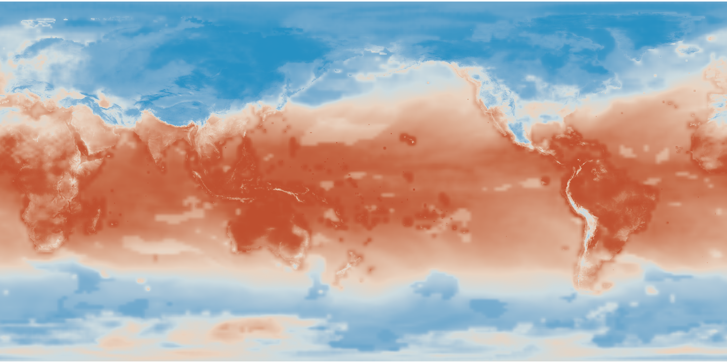
- A png of the first tile (the tile for day 0) in the given GDDP dataset, that will appear in
/tmp/gddp.png - A png of the first tile clipped to the extent of the GeoJSON polygon that was given, that will appear in
/tmp/gddp1.png - A png of the first tile clipped to the extent of the GeoJSON polygon and masked against that polygon, that will appear in
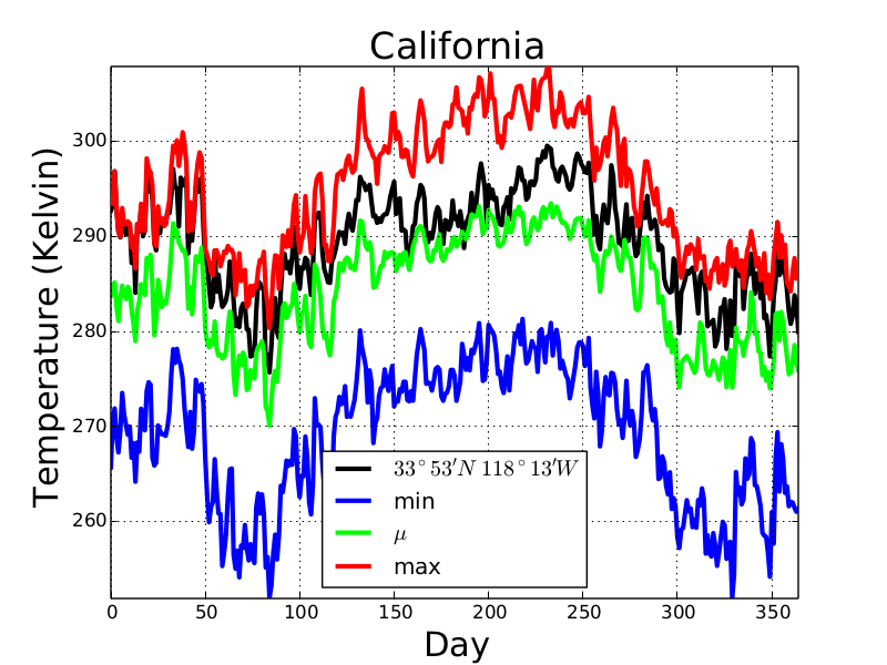
/tmp/gddp2.png - Time series of the minimum, mean, and maximum temperatures in the area enclosed by the polygon, as well as temperatures at the given point
Example 1 (Local File)
If you download the files3://nasanex/NEX-GDDP/BCSD/rcp85/day/atmos/tasmin/r1i1p1/v1.0/tasmin_day_BCSD_rcp85_r1i1p1_inmcm4_2099.nc , then type:\ and put it into a local file called /tmp/tasmin_day_BCSD_rcp85_r1i1p1_inmcm4_2099.nc
$SPARK_HOME/bin/spark-submit --master 'local[*]' \
   gddp/target/scala-2.11/gddp-assembly-0.22.7.jar \
   /tmp/tasmin_day_BCSD_rcp85_r1i1p1_inmcm4_2099.nc \
   ./geojson//CA.geo.json \
   '33.897,-118.225'
You will get the following results. The whole first tile:
The first tile clipped to the extent of the polygon (the boundary of California):

The first tile clipped and masked:

Here are the time series in graphical form. (The code in this project did not produce graph, just the data.)
This program should take about 10 seconds to complete.
Example 2 (File on S3)
We can re-run the same example, this time reading the data directly from S3:
$SPARK_HOME/bin/spark-submit --master 'local[*]' \
   gddp/target/scala-2.11/gddp-assembly-0.22.7.jar \
   's3://nasanex/NEX-GDDP/BCSD/rcp85/day/atmos/tasmin/r1i1p1/v1.0/tasmin_day_BCSD_rcp85_r1i1p1_inmcm4_2099.nc' \
   ./geojson//CA.geo.json \
   '33.897,-118.225'
The output will be the same as above, but the process will take longer to complete — generally about 2 minutes and 40 seconds in my experience. (Of course, this will vary with connection speed and proximity to the S3 bucket.)
Measurements show that about 190 – 200 megabytes are downloaded in total. Two separate sweeps are taken through the file (one to produce the clipped tiles and one to do point reads). The cost of taking one pass through the file — reading subsets of size 32 KB or less of each tile — is about 95 – 100 megabytes. (The file is 767 megabytes, the amount downloaded varies with the number of executors used.) There is still room for improvement in the S3 functionality, that is [discussed below](#future-work-better-s3-caching).
Structure Of This Code
In this section, we will address some of the key points that can be found in this code.
Open
def open(uri: String) = {
  if (uri.startsWith("s3:")) {
    val raf = new ucar.unidata.io.s3.S3RandomAccessFile(uri, 1<<15, 1<<24)
    NetcdfFile.open(raf, uri, null, null)
  } else {
    NetcdfFile.open(uri)
  }
}
is where the local or remote NetCDF file is opened. Notice that there are different code paths for S3 versus other locations; that is not strictly necessary, but is done only for efficiency.
NetcdfFile.open("s3://...") returns a perfectly workingNetcdfFile, but its underlying buffer size and cache behavior are not optimal for GDDP. That is further discussed below.
Whole Tile Read
val ncfile = open(netcdfUri)
val vs = ncfile.getVariables()
val ucarType = vs.get(1).getDataType()
val latArray = vs.get(1).read().get1DJavaArray(ucarType).asInstanceOf[Array[Float]]
val lonArray = vs.get(2).read().get1DJavaArray(ucarType).asInstanceOf[Array[Float]]
val attribs = vs.get(3).getAttributes()
val nodata = attribs.get(0).getValues().getFloat(0)
val wholeTile = {
  val tileData = vs.get(3).slice(0, 0)
  val Array(y, x) = tileData.getShape()
  val array = tileData.read().get1DJavaArray(ucarType).asInstanceOf[Array[Float]]
  FloatUserDefinedNoDataArrayTile(array, x, y, FloatUserDefinedNoDataCellType(nodata)).rotate180.flipVertical
}
This code is where the whole first tile (tile for day zero) is read into a GeoTrellis tile. Notice the assignments: latArray = vs.get(1)... lonArray = vs.get(2)..., and tileData = vs.get(2).... These are enabled by prior knowledge that in GDDP files, the variable with index 1 is an array of latitudes, the variable w ith index 2 is an array of longitudes, and the variable with index 3 is three-dimensional temperature data. Perhaps a more robust way to do that would be to iterate through the list of variables and match against the string returned by vs.get(i).getFullName( , but the present approach is good enough for government work. The dimensions of the temperature data are time (in units of days), latitude, and longitude, in that order. vs.get(3).slice(0, 0) vs.get(3).slice(0, 0) requests a slice with the first (0th) index of the first dimension fixed; it requests the whole tile from the first (0th) day. The assignment nodata = attribs.get(0).getValues().getFloat(0) gets the “fill value” for the temperature data which is used as the NODATA value for the GeoTrellis tile that is constructed.
Partial Tile Read
val array = tasmin
  .read(s"$t,$ySliceStart:$ySliceStop,$xSliceStart:$xSliceStop")
  .get1DJavaArray(ucarType).asInstanceOf[Array[Float]]
FloatUserDefinedNoDataArrayTile(array, x, y, FloatUserDefinedNoDataCellType(nodata)).rotate180.flipVertical
This code is where the partial tiles (matched to the extent of the query polygon) are read. Here, instead of using the slice method, the slicing functionality of the read method is used. The string that results from s"$t,$ySliceStart:$ySliceStop,$xSliceStart:$xSliceStop"will contain three descriptors separated by commas; the first is a time (specified by an integral index), the second is a latitude range (a range of integral indices with the start and end separated by a colon) and the last is a longitude range (again, a range of integral indices).
Point Read
tasmin
  .read(s"$t,$ySlice,$xSlice")
  .getFloat(0)
This code uses the slicing capability of the read method to get the temperature value at a particular time, at a particular latitude, and at a particular longitude. # Future Work: Better S3 Caching # As mentioned above, the efficiency of reading from S3 is an area for future improvement. There are many different types of files that have the extension .nc, in this brief
Future Work: Better S3 Caching
As mentioned above, the efficiency of reading from S3 is an area for future improvement. There are many different types of files that have the extension.nc , in this brief discussion we will restrict attention the GDDP dataset. Those files store the temperature data in compressed chunks of roughly 32 KB in size, and those chunks are indexed by a B-Tree with internal nodes of size 16 KB.
Within the S3 reader, a simple FIFO cache has been implemented. The S3RandomAccessFile implementation emulates a random access file, and for compatibility must maintain a read/write buffer. For simplicity, the cache block size used is twice the size of that buffer.
When one makes a call of the formNetcdfFile.open("s3://...") , the buffer size used is 512 KB which results in 1 MB cache blocks. That implies that every request to read an uncached datum incurs a 1 MB download. For many access patterns, such as reading random whole tiles, that is not a problem and in fact is the intended behavior. However, reading small windows or single pixels from different tiles is not a good access pattern for this scheme.
Such a pattern would result in a lot of extra data being downloaded and cached when accessing leaves, as well as the eviction of large cache blocks containing internals nodes (which presumably may be revisited) in favor of cache blocks containing (single-use) leaf nodes. The special-case that contains the line raf = new ucar.unidata.io.s3.S3RandomAccessFile(uri, 1<<15, 1<<24)creates an S3RandomAccessFile with a 32 KB read/write buffer and 64 KB cache blocks. The 64 KB cache blocks are a much better fit than the 1 MB ones that would have been created by default.
Examination of the access patterns generated by point queries, e.g. read("107,22,7"), shows that accesses are in general not aligned to block boundaries which frequently results in two blocks being fetched when one would have done. There is also the question of unnecessary cache eviction that was raised above. One of many ideas for improvement is to implement a cache that pays attention to the particular structure of the file rather than just managing blocks of bytes. That can potentially be done by inspecting the program state before a read is performed to determine whether the request is for an internal node or a leaf. If it is an internal node, the entire node can be cached (or returned from the cache), and if it is a leaf the request can be serviced without involving the cache.