
This Month We Learned (TMWL) is a recurring blog series inspired by a series of the same name at SoftwareMill. It gives us an opportunity to share short stories about what we’ve learned in the last month and to highlight the ways we’ve grown and learned both in our jobs and outside of them. This month we learned about principled ad hoc style variation with variants, handling too-big-for-memory data with Dask, and keeping long-term projects objective in mind while designing solutions.

Alex Lash 
Luke McKinstry Tai Wilkin


Rebass variants
Alex Lash
Balancing consistency with flexibility is always a challenge in web projects—especially when it comes to typography. Recently, we used Styled Components for a React app, and leveraged the Rebass framework’s variant prop to apply type styles. Here’s what we can do:

Rebass components come with some useful props by default, but our goals were to:
- establish some static properties,
- keep type styles in one location, so collaborators could easily import, alter, and refer to them, and
- change non-critical aspects on a case-by-case basis (e.g. invert the color on a dark background.)
Rebass allows us to use a theme.js file to set some relevant variables, such as fonts, sizes, and leading:
export default {
    font: 'Fira Sans, Helvetica, Arial, sans-serif',
    fontSizes: [
        '1.5rem', // 2
        '2.25rem', // 3
        '14rem', // 8
    ],
   fontWeights: {
        normal: '400',
        semibold: '600',
        black: '800',
    },
    lineHeights: {
        compact: '1',
        normal: '1.65',
        comfortable: '1.85',
    },
We can then make a Header.js file that imports everything we need to build out our type styles…
import { Heading as BaseHeading } from 'rebass';
import PropTypes from 'prop-types';
import styled, { css } from 'styled-components';
import { themeGet, style } from 'styled-system';
… and add two new propTypes for variant and fontStyle:
const variant = style({
    prop: 'variant',
    cssProperty: 'variant',
});

const fontStyle = style({
    prop: 'fontStyle',
    cssProperty: 'font-style',
});
Now we can make as many variants as makes sense for our project. Here are three heading styles for large, medium, and small variants of headings.
const Heading = styled(BaseHeading)${props => !!props.fontStyle && cssfont-style: ${props.fontStyle};}; ${props => props.variant === 'large' && cssfont-size: ${themeGet('fontSizes.8')}; font-weight: ${themeGet('fontWeights.normal)}; line-height: ${themeGet(lineHeights.compact')};}; ${props => props.variant === 'medium' && cssfont-size: ${themeGet('fontSizes.3')}; font-weight: ${themeGet('fontWeights.semibold)}; line-height: ${themeGet(lineHeights.compact)};}; ${props => props.variant === 'small' && cssfont-size: ${themeGet('fontSizes.2')}; font-weight: ${themeGet('fontWeights.black)}; line-height: ${themeGet(lineHeights.normal)};};;
Tip: anything you want to set for all styles but need to override in certain cases shouldn’t be written into the variant. Use defaultProps for those.
Heading.defaultProps = {
    color: 'black',
};
It’s a bit of setup, but now we can import the custom Header component to easily reference any of our font styles just by changing the variant prop. Best of all, thanks to the Styled Components as prop, we can easily use the semantically correct HTML element in our projects to make the GIF shown above.
Dask for medium-sized data
Luke McKinstry
This is an example of a solution for when data operations almost fit on your local machine.
Recently I was tasked with making GeoJSONs of Census statistics organized at the Block level (the most granular level of the Census hierarchy). This involves a lot of data for large states. For example, a GeoJSON of Census Blocks for Texas or California is larger than 1GB.
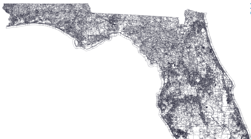
Here’s what the Census blocks look like for most of Florida:
GeoPandas is a popular tool at Azavea. However, joining my demographic statistics (in a Pandas DataFrame) and geographic boundaries (in GeoPandas GeoDataFrame) caused my machine to run out of memory. And it was generally slow for smaller states too.
To handle this task, I turned to Dask, a library for scaling data processing that sits on top of the well known Pandas/NumPy/Scikit-learn/Jupyter stack.
Leveraging existing Python APIs is great. This syntax to join 2 DataFrames, my desired task, will look familiar to Pandas users.
from dask import dataframe as dd
merge_dask_df = dd.merge(dask_df1, dask_df2, on=['colA','colB'])
One problem: Dask does not handle GeoDataFrames, which have a GeoSeries or geometry column that is a Shapely object for performing geometric operations in Python. We can solve this by converting the geo column to Well Known Binary (WKB) format, performing our Dask operations, converting WKB back to Shapely, and then resuming normal geographic operations.
The recommended best practices of Dask suggest reading and writing files from Apache Arrow format, so I use this workflow:
- Read census geographic files to GeoDataFrame, convert geometry to wkb, save locally in Apache Arrow format
- Read census demographic data to DataFrame, save locally in Apache Arrow format
- Read Apache Arrow files to Dask DataFrames, merge together, convert wkb back to geometry (in other words, convert Dask back to GeoPandas), perform other operations as needed
- Write to GeoJSON
Here’s what steps one and two look like:
import pandas as pd
import geopandas as gpd
from shapely import wkb

# geographic data
gdf = gpd.read_file(path_to_shapefile)
#convert geo column from Shapely to wkb (well known binary)
gdf["wkb"] = gdf.geometry.apply(lambda g: g.wkb)
gdf = gdf.drop(columns=["geometry"])
gdf.to_parquet(filepath_pyarrow_geo, compression='gzip' )

# demographic data
demo_df = pd.read_file(path_to_some_csv) #gathered from census api or file
demo_df.to_parquet( filepath_pyarrow_demo, compression='gzip' )
Here’s what steps three and four look like:
from dask import dataframe as dd

dask_df_geo = dd.read_parquet(filepath_pyarrow_geo, engine='pyarrow')
dask_df_demo = dd.read_parquet(filepath_pyarrow_demo, engine='pyarrow')
merge_dask_df = dd.merge(dask_df_geo, dask_df_demo, on=['census_geoid'])

# write dask df back to memory
back_to_mem_df = merge_dask_df.compute()
# convert wkb back to Shapely and drop wkb column
back_to_mem_df['geometry'] = back_to_mem_df['wkb'].apply(wkb.loads)
back_to_mem_df = back_to_mem_df.drop(columns=["wkb"])
# convert Dask back to GeoPandas
reformed_gdf = gpd.GeoDataFrame(back_to_mem_df, geometry='geometry')

# write GeoJSON
reformed_gdf.to_file( geojson_filepath , driver="GeoJSON" )
The final step, writing a huge GeoJSON, is still slow. However, now the entire process can be performed on a local machine thanks to Dask and Apache Arrow to scale the large intermediate join operations.
Maintainability thinking
Tai Wilkin
I was working on an issue that was small and contained (I thought). I produced a functioning polygonal search feature that sent a list of points to the backend to use as a reference to create a polygon and to return a filtered search result.
For a short-term project, this would have been enough. However, in the context of this long-term project, a more experienced developer pointed out that this solution needlessly limited us to a specific type of shape, when other options allowed for more flexibility.

In reformatting the data patterns to work with a more generalized GeoJSON, I had plenty of time to learn from the experience. I had initially considered the issue only in terms of the immediate needs of the task at hand, when, like in chess, there is always a larger context at play.
In order to advance as a developer, I need to improve in the same way as the chess player who sees only the move in front of them and is blind to the bishop waiting to take their pawn on the other side of the board. I learned, before beginning to work on any task, no matter the size, to stop and take a look at the whole board. How might we need to use this feature in five years?