
![]()
Recently, Azavea’s Data Analytics team was tasked with developing a GIS tool for the Delaware Division of Parks and Recreation to analyze level of service for the state’s recreational system. The goal of the project was to better understand what populations are being served by the system currently, and what areas are under-served. To equitably serve the people of Delaware, it’s only fair to consider all modes of transportation — such as walking and public transit, and this made the analysis much more complex. Basically, we needed to set up a tool that allows the DPR’s GIS department to input the type of recreation (such as playgrounds, basketball courts, swimming pools, etc.), buffer around those locations and summarize the population within those buffers. See our June newsletter for a detailed description of our model to distribute population.
We already knew that it makes sense to use travelsheds for this analysis, rather than the standard GIS buffer around a point. For this, we leveraged the Service Area analysis of the ArcGIS Network Analyst extension. The Service Area analysis will generate a polygon around a traversable feature, such as a street centerline, with a cost attribute such as time or distance as a parameter. This way, the DPR can generate polygons based on different times and distances — say a quarter mile from parks by walking or a 15 minute drivetime. We were able to successfully use the Delaware Department of Transportation’s (DelDOT) street centerline as an input for the driveshed portion of the service area analysis. In addition, the DPR provided a walkable roads shapefile that contained a mix of a sidewalk shapefile and roads with a low speed limit for generating the walksheds.
However, developing an accurate transit network for the Service Area analysis to traverse proved to be much more challenging. As it stands right now, ArcGIS does not have a way to read General Transit Feed Specification (GTFS) into Network Analyst. That being said, there is at least one plugin moving in that direction. Co-created by Melinda Morang, Product Engineer at Esri, the GTFS_NAtools python script allows users to run schedule-aware network analyses right in ArcMap. One can select the time of day and day of week and generate service areas based on what is traversable on the transit network. After some exhaustive testing and developing a workflow around the tool, we decided that the workflow was actually a bit too complicated for what we were trying to do. DPR didn’t need a time of day specific service area, just something more generalized but still with a reasonable travel time estimate.
Therefore, our team decided we would download the GTFS data and hardwire it into a transit network dataset. The first step would be to convert the GTFS data, which comes in the form of several comma-delimited text files, into a readable shapefile for an ArcGIS Network Dataset. Luckily, there’s already a great tutorial on how to do this. It only requires downloading the free ET GeoWizards toolbox, which every GIS Analyst should have at their disposal. Once finished, we ended up with a polyline for each individual bus route. However, it’s not quite ready to be consumed by Network Analyst. Since sometimes different bus routes use the same road, we had many coincident route segments. This creates a problem for the Service Area analysis in Network Analyst. The Service Area analysis locates an origin feature and creates a polygon around that feature by traversing the network dataset. When the origin feature for the service area is located along a route with coincident bus polylines, it only picks up one of the polylines and ignores the other features. This creates chunky and illogical service area polygons.
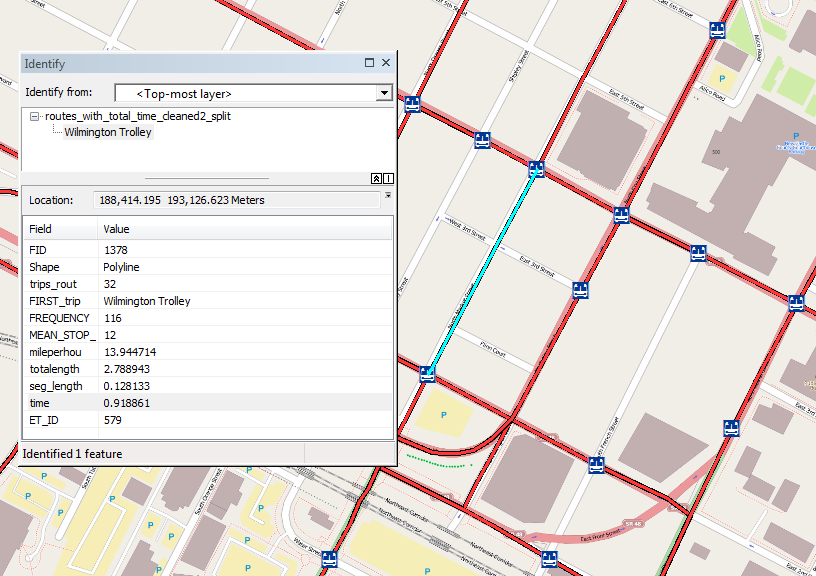
The solution we found was to flatten all the coincident bus polylines and create one bus routes polyline file that still maintained a best cost estimate of time for the Service Area analysis. In addition, we wanted to split the line at bus stops — that way service areas would be generated only around stops where people could actually get off the bus, rather than just along the line where bus riders cannot get on or off. The main challenge was to conflate bus travel times, which is maintained in the GTFS data, onto the bus routes. Since each bus route is divided into individual trips, we’d have to generalize the travel times a couple times to get what we wanted. Note that we used ET GeoWizards along the way, since some of the ArcGIS tools require more than the Basic (ArcView) license level. Though our toolbox for DPR is proprietary, we’re happy to share the methodology behind generating the bus routes with travel times. Here’s how to do it in 10 steps:
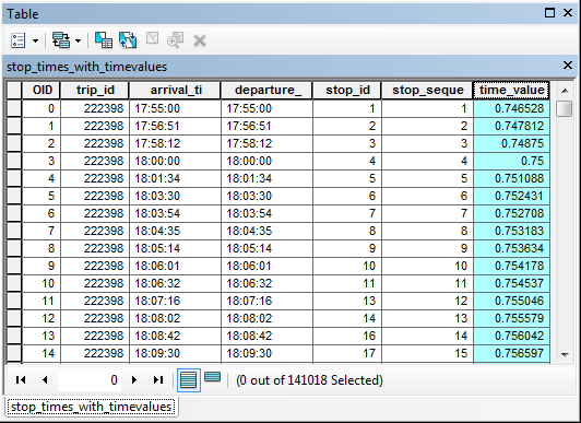
Step 1: This part involves finding the difference between the first stop and the last stop for each trip. That way we end up with a total time for each trip. To do that, bring the stop_times.txt file (comes with the GTFS download) into Excel and run the TIMEVALUE function on each of the stop times. Note that the file comes with an arrival and departure time. For DelDOT, this time was the same, so we just went with arrival time. The TIMEVALUE function calculates a decimal number value for each time of the day, with 0 being 12:00:00 AM and 0.999988426 (okay, pretty close to 1) for 11:59:59 PM. The new field is shown here, called time_value.
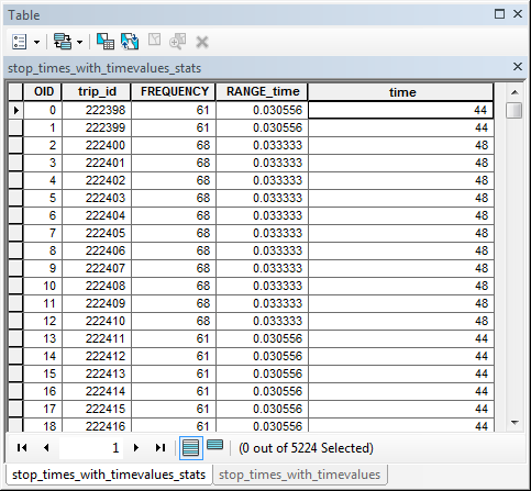
Step 2: Next, run Summary Statistics to find the total time for each trip. Taking the Excel file back into ArcMap requires a conversion to DBF to work with Summary Statistics.
Step 3: Add a field named time of type short integer. Using field calculator, multiply 1,440 (number of minutes in a day) by RANGE_time to get the total time in minutes for each trip.
Step 4: Join the trips table to bring over the route_id for each trip.
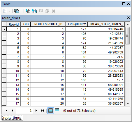
Step 5: Now, run summary statistics again using time as field with MEAN as statistic type and Case field route_id. At this point, we can join this to the routes shapefile and we’ve got a route file with travel time! We’re not done yet though, as we need to generalize the lines and split by bus stops.
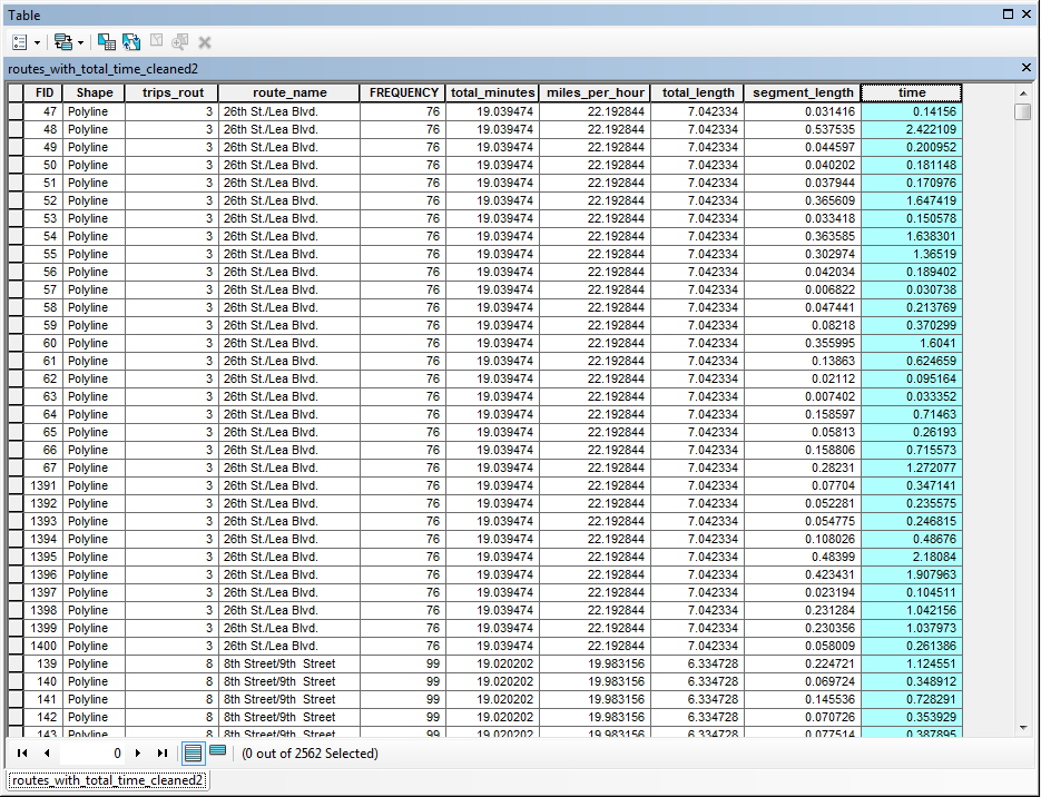
Step 6: Calculate the miles per hour for each bus route. To do this, add a field and populate it with the segment length in miles. Next, calculate the miles per hour that the bus travels along that line by using this formula. The minutes field is the total number minutes the bus takes to do the route that we created earlier.
60 / minutes * segment length
We’ll use this field after the next step to calculate new travel times on a cleaned layer.
Step 7: Run Clean Polyline Layer in ET GeoWizards. This removes redundant bus lines that overlap each other, leaving just one clean line for each route a bus travels down.
Step 8: Add a field called time and, using the miles per hour we generated in Step 6, calculate the time in minutes for each segment using Field Calculator. Use this formula:
segment length / miles per hour * 100
Step 9: Snap the points shapefile of bus stops to the bus routes. Use the Global Snap Points tool in ET GeoWizards. You can easily generate a points shapefile of bus stops using the latitude and longitude column in the stops.txt file that comes with the GTFS data.
Step 10: Split the bus routes file by the snapped bus stop points. Use the Split Polyline with Layer tool in ET GeoWizards. Select the option of “Proportion” for the time field. This will calculate a new time based on the shorter, split segments.
Finally, we’ve got a bus routes shapefile, split by bus stops with a value for bus travel time along each segment! Next, it’s ready to be converted into a Network Dataset for ArcGIS Network Analyst to build Service Area polygons.
It’s important to note some of the shortcomings with this approach. For one, there is a lot of generalization going on. The time values aren’t going to be highly accurate. Secondly, there is no ability to differentiate which bus route the user will take when feeding it into the Service Area analysis. However, since the finalized bus routes file has a route_id, one could easily extract just a particular route or set of routes to run an analysis on.
It was great to be able to use this project to experiment and learn about tools that we don’t often to get to use here at Azavea. We’re excited about the possibilities of using GTFS data with ArcGIS and hope to see what future versions of Network Analyst can do to make use of transit data. In the mean time, Melinda Morang’s collection of tools are fun to play around with but also have some exciting potential. In addition, we enjoyed assisting the DPR in using GIS to further the mission of providing recreation and parkspace to the great residents of Delaware. You can see the final results of this analysis in their Statewide Comprehensive Outdoor Recreation Plan.