At Azavea, we spend a lot of time helping our clients design and implement custom machine learning models (and writing open source software to make the process hurt a little less). We’ve built models to more efficiently route school buses, predict where crime is likely to occur during a police officer’s shift, and extract building footprints from satellite imagery. Without fail, every time we start a conversation with a new potential customer, one of the first questions we get is, “How accurate of a model can you make?” The answer is always the same, and typically disappoints: it depends.

• It depends on what your goals are (i.e. how this model will be used in real life). 
• It depends on how similar the project is to past work we’ve done. 
• It depends on the quality of training data we can generate or find. 
• Most of all, though, it depends on how we decide to define “accurate”.

In fact, after we create a model and measure it, we’re often still unsure of exactly how to describe its accuracy. There’s no shortage of ways to measure the performance of machine learning models, and I’ve tried to cover some of the most common and useful methods in this blog post. But in my experience, it’s harder to measure the accuracy of a machine learning model in the real world than it is to create it in the first place. Allow me to explain…

What is “Accuracy,” Technically?

To understand accuracy, you have to understand the four horsemen of the AI-pocalypse: true positive, false positive, true negative, and false negative. Collectively, these four measures describe the performance of most supervised machine learning models, and they’re pretty easy to grok. Imagine I’ve made a model that is searching photos for the greatest mascot in the history of modern civilization, Gritty. Here are four contrived examples of predictions that would fall into each category:

• 

• 

• 

• 

To get pedantic for a second, in the field of statistics, the term accuracy technically refers to a specific method of summarizing a model’s predictions according to those four categories:

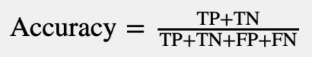
It feels very intuitive–you simply take all of the true predictions and divide those by the total number of predictions to get the accuracy. That seems reasonable enough, right? Wrong. In our case, accuracy is a terrible measure of accuracy. To illustrate:

Let’s say you’re capturing aerial imagery of a several-hundred mile stretch of pipeline, like our partners American Aerospace do routinely, and you’re looking for a needle in a haystack—some goober with a backhoe breaking ground on the cusp of causing a multi-million dollar environmental disaster. Most of the pipeline looks vast and empty:

You want a model that can localize construction equipment in real-time to save the day:

There’s a very low signal-to-noise ratio, which makes for a great machine learning project: a simple task for a human (identifying construction equipment in aerial imagery) that requires combing through an inhuman amount of data as quickly as possible. 

Given the goals of this challenge, if we were hired to build a model to automate this task, we would consider a good outcome to be a model that finds as close to 100% of the construction equipment in imagery as possible, even if that means it also spits out a decent amount of garbage predictions. The cost of missing a true positive is just too high, and even a relatively high ratio of false positives to true positives would result in an order of magnitude less imagery to manually comb through. Let’s say our model is shown 10,000 images and finds 100/100 instances of construction equipment, and also falsely predicts an additional 200 instances of construction equipment that are false alarms. We can plot that using something called a confusion matrix, and then run that through our accuracy equation:

	Positive Prediction	Negative Prediction
Positive Example	TP = 100	FP = 200
Negative Example	FN = 0	TN = 10,000

• 

• 

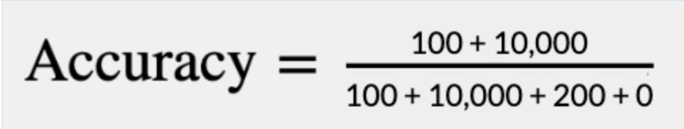
We’ve built a 98% accurate model! Pretty, pretty good. How could we possibly improve on a 98% accurate model? The easiest way would be to write a simple script that never predicts any construction equipment in any of the imagery it’s shown no matter what:

	Positive Prediction	Negative Prediction
Positive Example	TP = 0	FP = 0
Negative Example	FN = 100	TN = 10,000

• 

• 

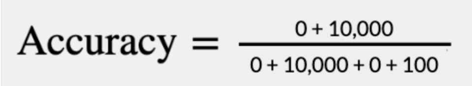
In this case, a worse-than-useless model is “more accurate” than an incredibly useful one. Why is that?

The Confounding Case of Class Imbalance 

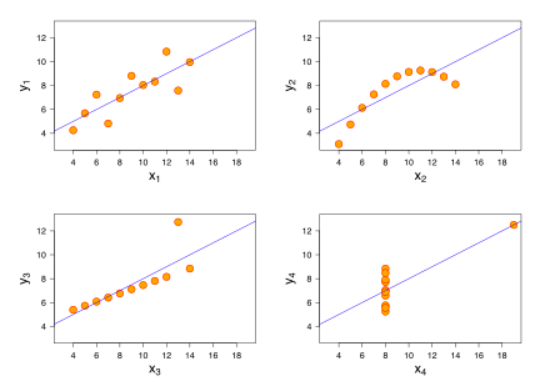
Class imbalance happens when the categories a model is trained to detect are unevenly distributed in the real world (which is almost always the case), and it’s one of the reasons we never use accuracy to describe the performance of machine learning models. It’s a special case of the more general concept in statistics of irregular distributions, which are famously deceptive if summarized haphazardly. The most famous illustration of this concept is Anscombe’s Quartet, which demonstrates four very different datasets that share the exact same summary statistics to a couple of decimal places.

A more recent (and fun) example is the Datasaurus Dozen from Autodesk research:

The point is: whenever you work to understand a complex dataset, like the range of outcomes from a machine learning model, you can’t really understand its performance by boiling it down to a few summary statistics. You have to look at the data yourself. Still, the reason people are excited about automation is that it can work at inherently inhuman scales, so sometimes you can’t feasibly look at even a small fraction of the data, which is why we still bother with summary statistics. Below are some of the more useful metrics we use to evaluate the models we create at Azavea, and the best part–underneath all of them are the same old concepts of true positive, false positive, true negative, and false negative predictions.

Precision & Recall

The simplest summary statistics to understand that actually are practical are precision and recall.

• Precision is the percentage of guesses a model makes that are correct. You can calculate precision with a simple formula: TP/(TP + FP). In the construction equipment detection example above, our 98% accurate model had a precision of 100/(100 + 200) = 0.33.
• Recall is the percentage of true positives that a model captured. The formula for recall is TP/(TP + FN). Our construction equipment model had a recall of 100/(100 + 0) = 1.0.

Precision and recall can be plotted against each other, and generally, share an inverse relationship. A trained model can be tweaked to favor precision or recall, without having to retrain it–you simply change the threshold of “confidence” the model has in a prediction up or down to move a model further left-or-right along the precision-recall curve:

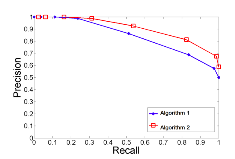
When we consult with clients, precision and recall are often useful ways of getting at the goals of a project, e.g., “Would you rather have a high-precision/low-recall model or a high-recall/low-precision model?”

F-Score (F₁ Score)

Often, the most salient metric we use is called F-Score, and it’s usually the closest thing to a stand-in for overall “accuracy” we share with clients. It’s less susceptible to the vagaries of class imbalance that accuracy suffers from, and it’s flexible enough to accommodate a client’s preference for precision vs. recall. Technically, it’s the harmonic mean of precision and recall:

Above is the equation for F₁ Score, where precision and recall are equally weighted. But there are any number of F-Scores; F_0.5 Score weights precision twice as much as recall, while F₂ Score weights recall as twice as important. Another strength of the F-measure is that it penalizes extremely poor performance in either category. If you compare three models and how they would be scored with a simple average of precision and recall vs. an F₁ Score, you can see what I mean. Model C has the best average of precision and recall, but is a deeply flawed model, while Model A is more balanced and scores better on its F₁ Score:

Model	Precision	Recall	Average	F1 Score
A	0.5	0.4	0.45	0.444
B	0.7	0.1	0.4	0.175
C	0.02	1.0	0.51	0.392

Advanced & Custom Metrics

If you start reading academic deep learning papers, you’ll run across a host of other metrics not discussed here–some we see a lot include average precision, mean average precision, the Jaccard Index (more commonly referred to as intersection over union), among others. The two most important aspects of choosing an evaluation metric are:

1. You are confident you understand what it’s describing.
2. It aligns with your goals, i.e. a higher score is truly a more valuable model.

In the ideal case, you can develop your own custom accuracy measure. One of my favorite examples of this is the first SpaceNet Road Detection Challenge, where a large dataset of labeled satellite imagery was released and a competition ensued to see who could extract the most accurate road network. The organizers (ComsiQ Works) were savvy enough to test out different evaluation metrics before announcing the competition and realized that F₁ Score wouldn’t be an effective tool for scoring submissions. Since they were comparing correct vs. incorrect predictions at a pixel level, the scoring algorithm couldn’t account for the utility of bothering to extract a road in the first place–something that is navigable and connected to a graph of other roads. So submissions that were splotchy but captured the whole road (more useful as a precursor for mapping a road network) scored worse than delicate but spotty predictions:

So they came up with their own scoring system, the Average Length Path Similarity (APLS) metric. It actually tries to navigate the optimal path between two points in the road network (first on the ground truth, then on the predicted road network) and compares the differences between the two. Predictions that artificially leave gaps in the road network where there shouldn’t be gaps are penalized, and more navigable networks are rewarded. The result is a much less intuitive absolute metric (no one has ever bragged that their model scored a 0.2 on the APLS metric) but a much fairer and more useful way to assess the performance of the models that were submitted to them as part of that competition:

The Big Takeaways

The best way to think about metrics used to describe the “accuracy” of machine learning models is to understand them as comparative tools, not as absolute measures. 

The reason these metrics were invented in the first place was so that researchers could better understand if they were getting “better” or “worse” as they iteratively tried different algorithmic approaches to problems. A model with an F₁ Score of 0.98 is not 98% accurate, exactly, but it’s probably more trustworthy than a model trying to accomplish the same task that has a much lower F₁ Score. 

If you want to understand how accurate a model is, look at its predictions directly, not at its summary statistics.

There is no substitute for the instincts you can gain about a model by simply looking at its output directly. Like Anscombe’s Quartet, the devil is in the distribution.

All models have strengths and weaknesses–you should be able to describe both.

There is no such thing as a 100% accurate model, it’s a philosophical impossibility. In fact, I wrote a whole blog post about it! So a good rule of thumb, when evaluating models, is to think about them as inherently flawed prediction engines that are editorialized to prefer making certain kinds of mistakes over others. Whether that’s weighting a model toward recall vs. precision or limiting its use to a certain subset of data that it performs better on, you are being irresponsible if you can’t talk about specific tradeoffs that you’ve made when designing a model.